
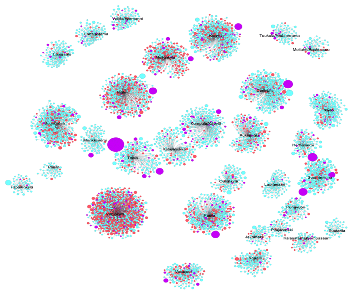
Figure 1
Observed racial composition of all groups (n = 6,496).

Figure 2
Observed racial composition of groups observed in the district of Vartiokylä.
Table 1
Results of logistic regression model predicting racial heterogeneity in a group from other group attributes.
| ESTIMATE (SE) | p | |
|---|---|---|
| Intercept | –2.23 | |
| Gender (ref = female group) | ||
| Male group | 0.25 (0.16) | 0.115 |
| Mixed-gender group | 0.54 (0.15) | 0.0003 |
| Age (ref = 0–14 years) | ||
| 15–18 | –0.30 (0.21) | 0.143 |
| 19–30 | –0.69 (0.19) | 0.0004 |
| 31–45 | –1.26 (0.22) | <0.0001 |
| 46–64 | –2.68 (0.39) | <0.0001 |
| 65+ | –3.72 (0.60) | <0.0001 |
| Adults and children/teens | –2.11 (0.20) | <0.0001 |
| Adults and adults | –1.46 (0.25) | <0.0001 |
| Group size (ref = 2 people) | ||
| 3 people | 0.61 (0.15) | <0.0001 |
| 4 people | 1.41 (0.19) | <0.0001 |
| 5–7 people | 1.22 (0.28) | <0.0001 |
| 8+ people | 3.17 (0.43) | <0.0001 |
| Time of day (ref = 9–12) | ||
| 12–16 | 0.33 (0.20) | 0.095 |
| 16–19 | 0.25 (0.21) | 0.234 |
| 19–> | 0.44 (0.27) | 0.106 |
| Area income (ref = lowest Q) | ||
| Second quartile | 0.08 (0.14) | 0.569 |
| Third Q quartile | –0.16 (0.23) | 0.489 |
| Fourth Q quartile | –0.59 (0.19) | 0.002 |
| Public place (ref = public) | ||
| Not public | –0.04 (0.18) | 0.804 |
[i] Note. Unstandardized estimates are presented. Pseudo-R-squared (calculated via McFadden’s method) was 0.24. And 95% confidence levels for all contrast estimates are presented in Table S4. Income quartile limits were (in euros per household on average) 48,767, 54,519, 67,874, and 102,347.
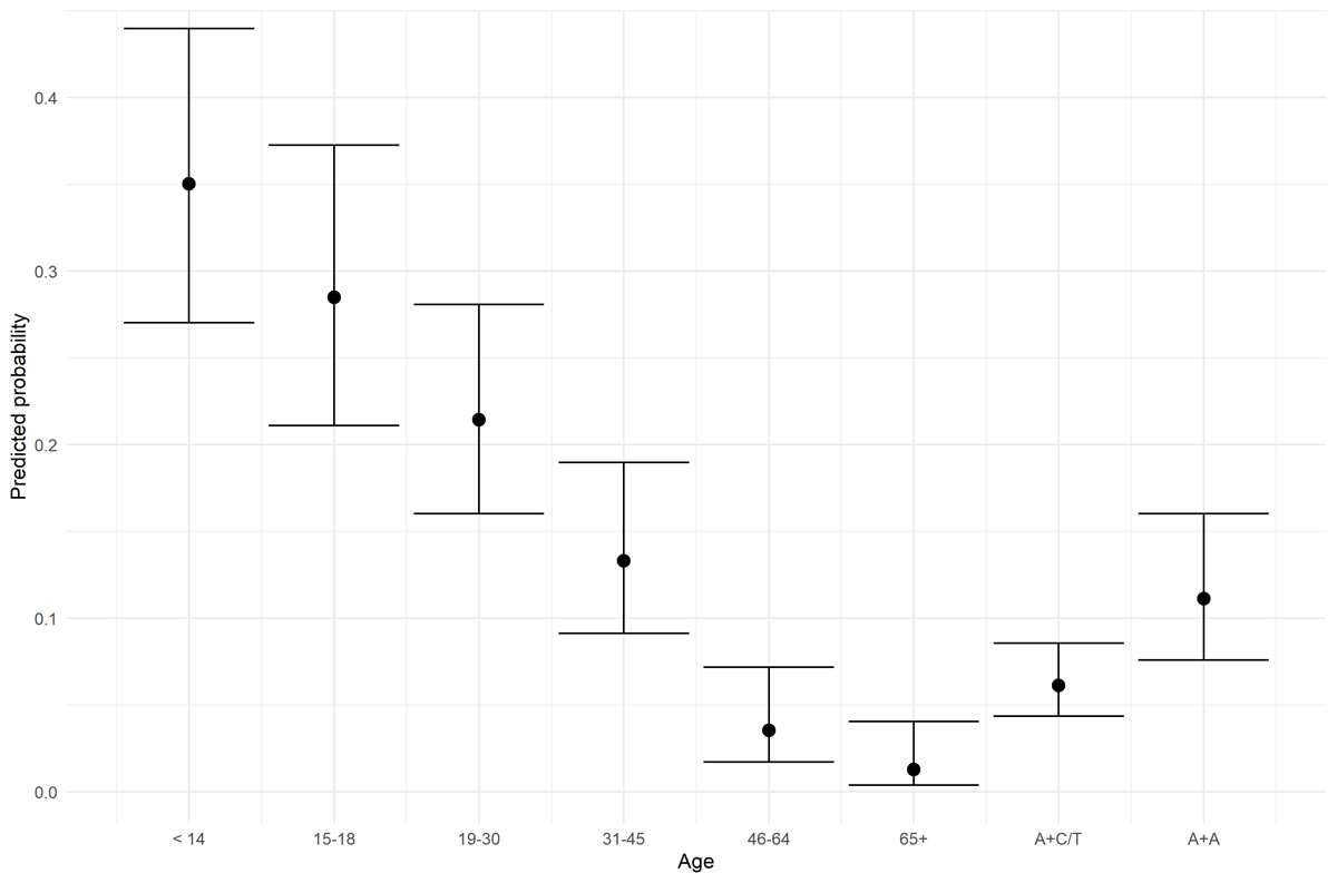
Figure 3
Predicted probabilities of observed racial heterogeneity in a group per age group, with 95% confidence levels. A + C/T = Adults with children and/or teens. A + A = Adults from different age groups.
Table 2
Results from a logistic regression model predicting group’s nighttime (after 7 pm) appearance from group gender composition, group racial composition, and their interaction.
| B (SE) | p | |
|---|---|---|
| Intercept | –3.02 | |
| Gender comp. (ref = female) | ||
| Male group | 0.01 (0.26) | 0.971 |
| Mixed-gender group | 0.73 (0.37) | 0.047 |
| Racial comp. (ref = all-White group) | ||
| All non-White group | 0.17 (0.19) | 0.368 |
| Mixed race group | 0.48 (0.14) | <0.001 |
| NW × Male | 1.05 (0.32) | 0.001 |
| Mixed Ethn × Male | –0.73 (0.58) | 0.206 |
| NW × Mixed-Gender | –0.10 (0.32) | 0.764 |
| Mixed ethn. × Mixed-Gender | –0.05 (0.44) | 0.904 |
[i] Note. Unstandardized coefficients are presented. For pairwise contrasts (with confidence levels), see Table S6. Pseudo-R-squared (computed via McFadden’s method) was 0.02.

Figure 4
Nighttime appearance as a function of group gender and ethnic composition.
Table 3
Fit indices for the latent class solutions.
| AIC | BIC | SABIC | ENTROPY | |
|---|---|---|---|---|
| Two classes | 58,315.32 | 58,538.87 | 58,434.01 | 0.74 |
| Three classes | 57,646.42 | 57,985.13 | 57,826.25 | 0.66 |
| Four classes | 57,160.81 | 57,614.69 | 57,401.79 | 0.66 |
| Five classes | 57,015.53 | 57,584.58 | 57,317.65 | 0.64 |
| Six classes | 56,898.51 | 57,582.71 | 57,261.75 | 0.73 |
[i] Note. SABIC = sample-size adjusted BIC.
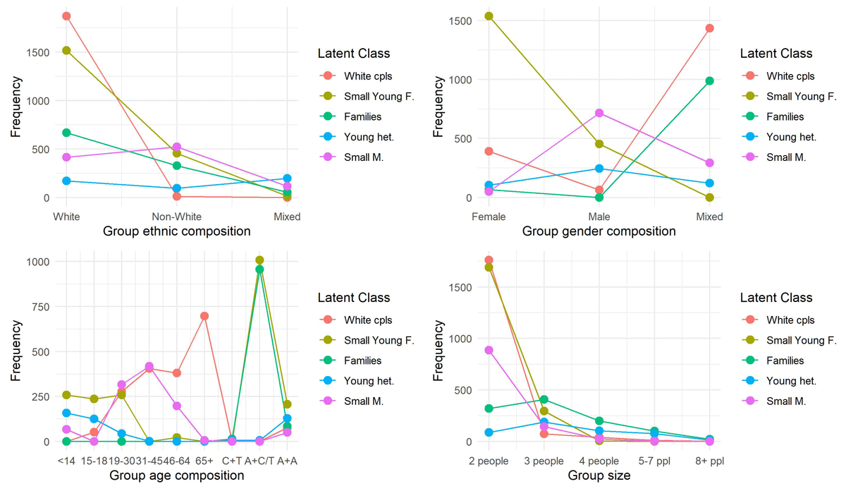
Figure 5
Frequencies of indicator levels in the 5-cluster solution.
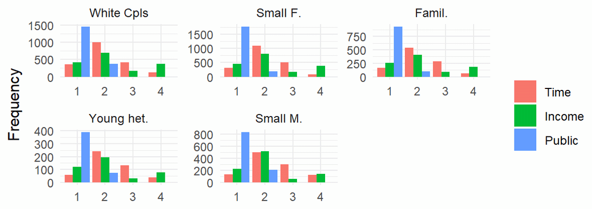
Figure 6
Frequencies of clusters at different times, in dirrernt income areas and in public vs. not public places.
Note. For ‘public’, 1 = public and 2 = not public.