For much of the modern investment era, long-dated U.S. Treasury securities have been viewed as a natural hedge for equity risk, a premise that underpins the classic 60 percent equity / 40 percent bond portfolio. The argument rests on the empirical observation that equity and Treasury return tend to move in opposite directions, so that bond rallies offset stock-market drawdowns and reduce overall portfolio volatility (Campbell and Viceira, 2002). Yet, it is clear that this negative co-movement is neither constant nor guaranteed.
The high inflation episode of 2022–23 calls the stability of this relationship into question. As headline inflation surged, the Federal Reserve responded with aggressive monetary tightening. Both the S&P 500 and long-duration Treasuries suffered double-digit annual losses, and the rolling sixty-day stock–bond correlation turned decisively positive. Whether this joint sell-off represents a fleeting anomaly or signals a durable regime change is a question of immediate importance to asset allocators, risk-parity managers, and policymakers who have long relied on Treasuries for diversification.
This study offers a formal econometric test of that question. The central hypothesis is that the 2022–2023 period constitutes a structurally distinct, inflation-dominated regime in which U.S. Treasuries lose their diversifying power. Using a two-state Markov-Switching model, this paper endogenously identifies “Calm” and “Crisis” regimes for both stocks and bonds from 2007 to 2023. By comparing the characteristics of these regimes across the Global Financial Crisis of 2008, the COVID-19 crash of 2020, and the inflation-driven downturn of 2022, this research aims to provide a clean, quantitative comparison of these events and contribute fresh evidence to the ongoing discussion about the stability of the classic portfolio hedge.
The remainder of the paper is organised as follows. Section 2 reviews the relevant literature on the drivers of the stock-bond correlation and the methods used to analyze it. Section 3 describes the Markov-Switching methodology. Section 4 details the empirical data used in the analysis. Section 5 presents and discusses the empirical results. Section 6 concludes and outlines directions for future research.
The traditional 60/40 portfolio allocation strategy has long been predicated on a stable, typically negative, correlation between stocks and bonds, where bonds provide diversification benefits during equity market downturns (Campbell and Viceira, 2002). However, extensive research suggests this relationship is neither constant nor predictable, exhibiting significant time-variation and regime-dependent behavior.
The relationship between stock and bond returns has undergone dramatic regime shifts throughout history, with correlation patterns revealing fundamental changes in economic conditions and investor behavior over more than a century of market data (Brixton et al., 2023).
During the early 20th century through the 1960s, correlations were generally positive, averaging around +30%, as both asset classes responded similarly to economic cycles under relatively stable monetary systems, though notable exceptions occurred during crisis periods like the Great Depression (1929–1932) when flight-to-quality dynamics produced negative correlations (Molenaar et al., 2023).
Baele et al. (2010) also confirm that correlations have oscillated widely, being positive in the 1970s and deeply negative after 1998 with numerous structural breaks at identifiable historical junctures (Fang et al., 2018). The period from 1965 to 1997 marked an era of strongly positive correlations, reaching extreme levels of +50% to +70% during the 1970s oil crises and stagflation, when both stocks and bonds suffered simultaneously from double-digit inflation and aggressive monetary policy responses under Federal Reserve Chairman Paul Volcker in the early 1980s (Brixton et al., 2023). A critical regime shift occurred around 2000 with the dot-com bubble burst (Naresh et al., 2014), initiating a 20-year period of consistently negative correlations averaging −30%, characterized by low and stable inflation, growth-focused central bank policies, and bonds serving as effective portfolio hedges during equity downturns including the 2008 Financial Crisis (Vatsa et al., 2024). The Global Financial Crisis and the COVID-19 pandemic represent other pivotal moments that triggered significant changes in correlation patterns (Cai et al., 2021). This historical perspective is crucial for understanding potential structural changes, as the assumption of a stable relationship may be fundamentally flawed.
Research consistently identifies macroeconomic variables and market-based factors as the fundamental drivers of stock-bond correlation dynamics. The prevailing theoretical explanation hinges on the relative importance of growth versus inflation shocks (Campbell et al., 2021). Economic growth shocks typically move stocks and bonds in opposite directions, fostering a negative correlation (Yang et al., 2009). In contrast, inflation shocks, such as the cost-push pressures seen in 2022–2023, tend to move both asset classes in the same direction as rising interest rates negatively impact both bond prices and stock valuations (Cieslak and Pflueger, 2023). The interaction between monetary and fiscal policy also fundamentally shapes correlation patterns (Li et al., 2022). Furthermore, market volatility, often measured by the VIX index, exhibits a sophisticated nonlinear relationship with the correlation, producing different outcomes in low-volatility environments compared to high-stress “flight-to-safety” episodes (Adrian et al., 2017). The COVID-19 pandemic provided valuable insights, with studies showing that sentiment indicators significantly influenced correlations, suggesting that behavioral factors play an increasingly important role during periods of elevated uncertainty (Banerjee, 2022).
To capture the complex dynamics of the stock-bond relationship, the literature employs a diverse set of sophisticated quantitative methods. Time-varying correlation models, particularly Dynamic Conditional Correlation (DCC) GARCH models, are extensively used to estimate conditional correlations that evolve over time (Adams et al., 2017; Banerjee, 2022). These have proven useful for analyzing correlation dynamics during crisis periods, where correlations tend to increase and compromise diversification. Vector Autoregression (VAR) models and their extensions represent another cornerstone of empirical analysis, allowing researchers to examine the dynamic interactions between multiple financial and macroeconomic variables simultaneously (Gao et al., 2023). For analyzing long-run equilibrium relationships, Vector Error Correction Models (VECM) have been particularly valuable when cointegration is present. Regime identification techniques are critical for understanding abrupt structural changes (Gao et al, 2025). Markov-switching models, following the seminal work of Hamilton (1989), remain popular for their ability to endogenously identify distinct correlation regimes based on data characteristics (Guidolin and Timmermann, 2006; Ang and Bekaert, 2002). These models have been particularly effective in showing that correlation regimes can persist for extended periods before undergoing abrupt transitions, often coinciding with major economic shocks. More recent approaches have begun to incorporate machine learning techniques to enhance regime identification (Wu et al., 2022). This study employs the well-established Markov-switching framework to provide a clear, interpretable analysis of the 2022–2023 regime shift.
The evidence of an unstable stock-bond correlation (Molenaar et al., 2024) has profound implications for portfolio management. The 2022 inflation surge and subsequent monetary policy tightening triggered one of the largest drawdowns for U.S. 60/40 portfolios in the last century, highlighting the limitations of static allocation strategies. Research indicates that dynamic, regime-aware allocation strategies can significantly improve risk-adjusted returns compared to static balanced portfolios (Kim and Kwon, 2023). This has led to an increased emphasis on the role of alternative assets, such as commodities and inflation-protected securities, as potential hedging instruments during periods when stock-bond correlations become positive (Page and Panariello, 2018), although their effectiveness also appears to be time-varying. Ultimately, the literature provides compelling evidence that investors and portfolio managers must move beyond static allocation models toward dynamic frameworks that can adapt to changing correlation environments.
The analysis proceeds in two stages: a preliminary exploratory analysis followed by the econometric modelling. First, an exploratory analysis was conducted using cumulative performance charts, rolling correlations, and an annual correlation heatmap to visualize the data and motivate the analysis. Second, a formal econometric model was implemented. To capture the discrete, time-varying nature of asset return dynamics, we employ a univariate two-state Markov-switching model, following the framework pioneered by Hamilton (1989). It assumes the return process is governed by an unobserved state variable that switches between two regimes, allowing the mean and variance to differ in each state. This model is particularly well-suited for identifying distinct market regimes, such as periods of low versus high volatility, without requiring a priori identification of structural break dates. The model is fitted independently to the stock (SPY) and bond (TLT) return series. This approach allows the data to endogenously identify periods of “Calm” versus “Crisis” for each asset class, which can then be compared over time to understand their joint behavior.
Let rt denote the asset r return at time t. The model assumes that the data-generating process for rt is dependent on an unobserved discrete state variable St, which can take one of two values, St ∈ {1,2}. Conditional on the state at time t, the return is assumed to be normally distributed with a state-dependent mean and variance. The model can be specified as:
This can be expressed as:
The unobserved state variable, St, is assumed to follow a first-order, discrete-time Markov chain. This process is defined by the trasition probabilities, which govern the probability of moving from one state to another in a single time step. The transition probability of moving from state i at time t − 1 to state j at time t is given by:
These probabilities are collected in a 2x2 transition probability matrix, P:
Since the state variable St is unobserved, the model's parameters must be estimated via Maximum Likelihood Estimation (MLE). The vector of parameters to be estimated θ = (μ1, μ1, σ1, σ1, p, q).The log-likelihood function is constructed recursively using a nonlinear filter, as developed by Hamilton (1989). The log-likelihood function is specifed as:
The estimation is carried out using the Expectation-Maximization (EM) algorithm, which iteratively updates the parameter estimates and the state probabilities until convergence. Upon estimation, the procedure yields not only the parameter estimates in θ̂, but also the filtered probabilities P(St = j ∣ Ft) and the smoothed probabilities, P(St = j ∣ FT), which represent the full-sample inference of the probability of being in state j at time t. These smoothed probabilities are used to classify each observation into one of the two regimes.
The analysis is based on daily data spanning from January 1, 2007, to December 29, 2023. This period was deliberately chosen to encompass multiple economic cycles, including the Global Financial Crisis, the COVID-19 pandemic, and the recent inflationary surge. To represent the core asset classes of a traditional balanced portfolio, this study utilizes highly liquid and widely recognized exchange-traded funds (ETFs) as proxies. The U.S. equity market is represented by the SPDR S&P 500 ETF (SPY), while the long-duration U.S. government bond market is represented by the iShares 20+ Year Treasury Bond ETF (TLT). The latter was specifically chosen for its high sensitivity to changes in inflation expectations and monetary policy. Adjusted closing prices were sourced from FMP Cloud data platform, from which daily logarithmic returns were calculated. To provide economic context for the identified market regimes, key macroeconomic variables were incorporated from the St. Louis Federal Reserve's FRED database, namely the Consumer Price Index (CPI) and the Effective Federal Funds Rate.
A preliminary visual inspection of the data reveals the unprecedented nature of the Inflation Crisis (from 2022-01-01 to 2023-12-29) market environment and provides motivation for a regime-based analysis. Figure 1 plots the cumulative performance of the S&P 500 (SPY), 20+ Year Treasury Bonds (TLT), and a hypothetical 60/40 portfolio on a logarithmic scale from 2007 to 2023. The chart clearly illustrates the traditional hedging relationship during the Global Financial Crisis (from 2008-09-15 to 2009-03-09) and the COVID-19 crash (from 2020-02-19 to 2020-04-30), where the bond market rallied, providing a crucial buffer against equity losses. However, a stark divergence from this pattern is evident in 2022, where both asset classes experienced significant and simultaneous declines, leading to the worst performance for the 60/40 portfolio in the entire sample period.
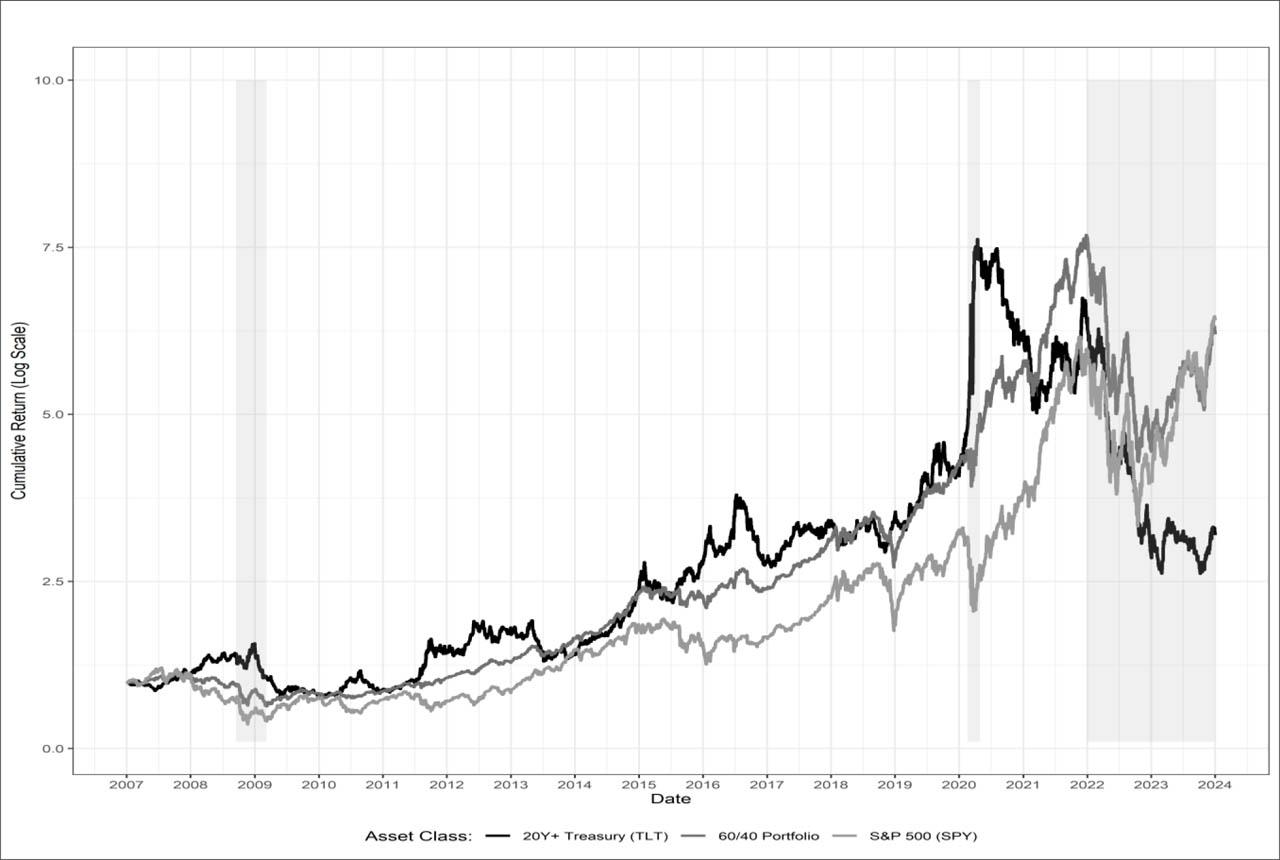
Cumulative performance: stocks, bonds, and 60/40 portfolio
Source: Author.
To more directly examine the underlying relationship, an annual correlation heatmap is presented in Figure 2. This visualization simplifies the noisy daily comovements into a clear year-over-year summary. The heatmap shows a consistent pattern of negative correlation for every year from 2007 through 2021. The years 2022 and 2023 represent a stark visual break from this long-standing trend, as they are the only two years in the entire sample to register a positive annual correlation between stocks and bonds. This provides strong first evidence of a structural shift in the comovement of the two asset classes.
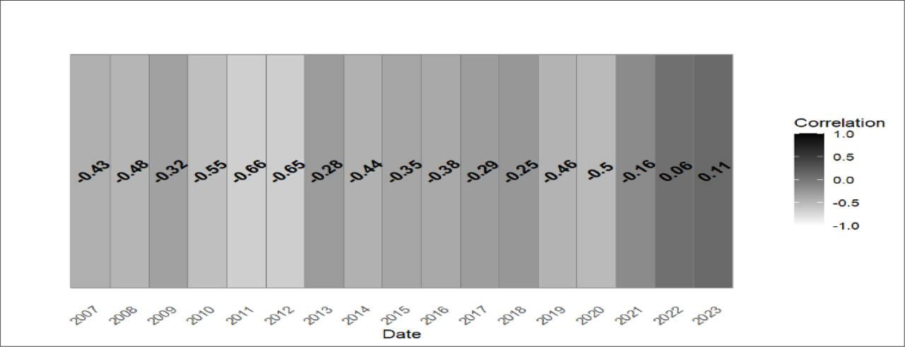
Annual stock-bond correlation heatmap
Source: Author.
A preliminary visual inspection of the dynamic relationship between U.S. stocks and Treasury bonds provides strong motivation for a regime-based analysis. Figure 3 plots the rolling Pearson correlation coefficient between the daily returns of SPY and TLT over multiple window lengths (30, 60, and 90 days) from 2007 to 2023. The chart reveals several distinct patterns. For the majority of the period prior to 2022, the correlation remains predominantly negative, oscillating around an average well below zero. During established crisis periods, such as the Global Financial Crisis (shaded area around 2009) and the COVID-19 crash of 2020, this negative correlation intensifies, with the correlation plunging towards its lowest levels in the sample. This illustrates the classic “flight-to-safety” dynamic where bonds act as a strong hedge against equity downturns. However, beginning in late 2021 and persisting through 2022 and 2023 (final shaded area), a clear break emerges. The correlation surges into positive territory and remains there for the most sustained period in the entire dataset, frequently exceeding +0.4. The close tracking of the different window lengths confirms that this is a robust phenomenon, not an artifact of the measurement period. This visual evidence strongly suggests the existence of at least two distinct correlation regimes, motivating the use of a formal Markov-Switching model to identify and characterize them.
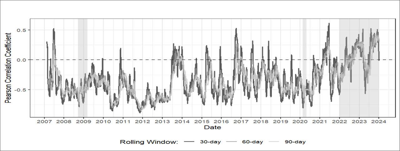
Rolling correlation between S&P 500 and 20Y+ treasury returns
Source: Author.
Before specifying the formal econometric model, several prespecification tests were conducted to justify the use of a non-linear, regime-based framework over a simpler linear model. The preliminary visual inspection of the data, particularly the rolling correlation plot shown in Figure 3, provides the initial motivation. The clear structural instability and time-varying nature of the stock-bond relationship suggest that a model assuming a constant correlation would be fundamentally misspecified. To formally test for non-linearities present in financial data, Engle's ARCH-LM test was performed to detect time-varying volatility, a phenomenon often described as volatility clustering. The test results for both SPY (p < 0.001) and TLT (p < 0.001) returns strongly reject the null hypothesis of no ARCH effects. This indicates the presence of significant conditional heteroskedasticity, confirming that a model assuming constant variance is inadequate. Furthermore, the unconditional distribution of the return series for normality using the Jarque-Bera test was tested. The null hypothesis of normality was also strongly rejected for both SPY (p < 0.001) and TLT (p < 0.001) returns, with both series exhibiting the characteristic excess kurtosis or fat tails common to financial assets. This non-normality provides additional motivation for a model capable of capturing different distributional properties across states, such as a multi-regime framework. Collectively, these preliminary findings build a robust case that a static, linear model is inappropriate for this analysis and that a more sophisticated approach, such as the Markov-Switching model, is required to adequately capture the underlying data generating process.
The formal econometric modelling confirms and extends the findings of the exploratory analysis. The Markov-Switching models (MSM) successfully identified two statistically distinct and economically interpretable regimes for both the equity and bond markets. The estimated parameters for each regime, presented in Table 1, allow for a clear characterization of the market states. For the SPY (Table 1), the model distinguishes between a “Bull Market” state (Regime 2), characterized by a positive mean daily return (0.108%) and low volatility (0.670%), and a “Bear/Crisis” state (Regime 1), defined by a negative mean daily return (−0.131%) and significantly higher volatility (2.063%).Similarly for the 20+ Year Treasury market (Table 2), the model identifies a “Safe Haven” regime (Regime 1), characterized by positive returns (0.026%) and low volatility (0.693%), and a “Hedge Failure” regime (Regime 2), defined by negative mean returns (−0.006%) and high volatility (1.304%). A key finding from the transition probabilities is the high degree of persistence in all identified states. The “Bear/Crisis” regime for equities, for instance, has an expected duration of approximately 23 trading days, while the “Hedge Failure” regime for bonds has an expected duration of 75 trading days, indicating that these states are not fleeting but represent sustained periods of market stress.
Estimated regime characteristics for SPY and TLT daily returns
| Asset | Regime | Return | Volatility | Persistence | Duration (days) |
|---|---|---|---|---|---|
| SPY | Regime 1 | −0.131 | 2.063 | 0.956 | 22.64 |
| Regime 2 | 0.108 | 0.670 | 0.981 | 52.36 | |
| TLT | Regime 1 | 0.026 | 0.693 | 0.992 | 127.87 |
| Regime 2 | −0.006 | 1.304 | 0.987 | 74.6 |
Source: Author.
Transition probability matrix
| S&P 500 (SPY) regimes | ||
| Regime 1 (Bull) | Regime 2 (Crisis) | |
| Regime 1 (Bull) | 0.9558 | 0.0191 |
| Regime 2 (Crisis) | 0.0442 | 0.9809 |
| 20Y+ Treasury (TLT) regimes | ||
| Regime 1 (Bull) | Regime 2 (Crisis) | |
| Regime 1 (Bull) | 0.9922 | 0.0134 |
| Regime 2 (Crisis) | 0.0078 | 0.9866 |
Source: Author.
The dynamics of the switching process between regime states in the MSM are governed by the transition probability matrices, presented in Table 3 for the S&P 500 and 20Y+ Treasury. These matrices quantify the persistence of each regime. For the S&P 500, the probability of remaining in the “Crisis” regime from one day to the next is 0.9809, while the probability of remaining in the “Bull” regime is 0.9558. Similarly, the bond market regimes exhibit even greater persistence, with probabilities of 0.9866 and 0.9922 of remaining in the “Crisis” and “Bull”, respectively. The high values of these diagonal elements confirm the strong persistence or stickiness of all identified regimes, validating the earlier finding of their significant expected durations. The small off-diagonal elements, in turn, represent the low daily probability of a switch occurring, underscoring that shifts between market states, while impactful, are relatively infrequent events.
Annual regime statistics for SPY
| Year | Average crisis regime probability (%) | % Days in crisis regime |
|---|---|---|
| 2007 | 30.9 | 28.0 |
| 2008 | 75.3 | 76.3 |
| 2009 | 61.1 | 59.9 |
| 2010 | 38.5 | 37.3 |
| 2011 | 46.3 | 44.0 |
| 2012 | 9.8 | 9.6 |
| 2013 | 4.8 | 3.6 |
| 2014 | 9.2 | 7.9 |
| 2015 | 18.8 | 19.8 |
| 2016 | 17.9 | 17.9 |
| 2017 | 0.1 | 0.0 |
| 2018 | 31.8 | 30.7 |
| 2019 | 10.5 | 8.7 |
| 2020 | 50.0 | 49.0 |
| 2021 | 13.8 | 13.1 |
| 2022 | 84.7 | 86.9 |
| 2023 | 9.1 | 6.8 |
Source: Author.
The central output of the MSM model is the time series of smoothed probabilities, which provides a data-driven historical record of when the market was in a particular regime. Figure 4 plots the MSM smoothed probability of the SPY being in its “Crisis” state. The plot demonstrates the MSM ability to endogenously identify well-known periods of market turmoil, with the probability spiking to nearly 100% during the GFC, the COVID-19 crash, and the 2022 downturn.
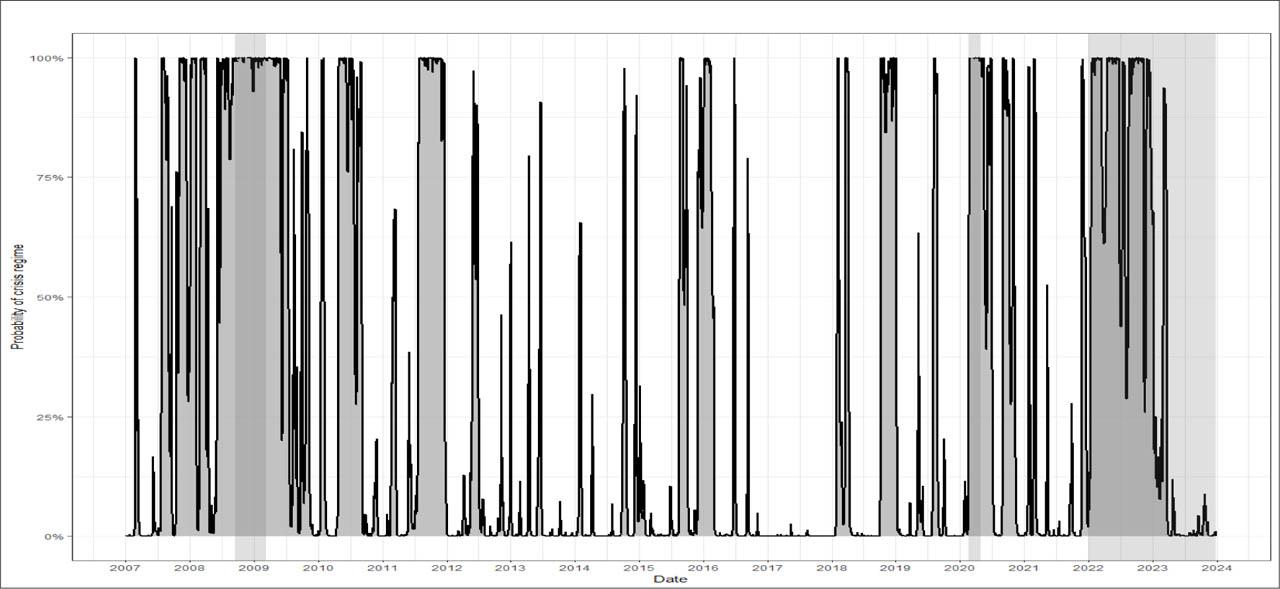
SPY crisis regime probabilities
Source: Author.
To quantify this, Table 3 presents the annual average breakdown probabilities of the MSM. The data reveal that 2022 was the most persistently turbulent year for equities in the entire sample period, with an average crisis probability of 84.7%. This figure is notably higher than that of 2008 (75.3%) and 2020 (50.0%), establishing the 2022 market downturn as a statistically significant crisis event. This finding is crucial, as it provides a common basis of equity market stress from which to compare the divergent behavior of the bond market across different crises.
To ensure these findings are not unique to long-duration bonds, a sensitivity analysis was conducted by replicating the Markov-Switching model using a medium-term bond proxy, the iShares 7–10 Year Treasury Bond ETF (IEF). The results were highly consistent. The model for IEF also identified a 'Hedge Failure' regime characterized by negative returns and high volatility. The smoothed probabilities for this regime spiked to nearly 100% during the 2022–2023 inflation shock, mirroring the results from the 20+ year bond analysis. This confirms that the inflation-driven breakdown of the stock-bond hedge was a broad phenomenon across the U.S. Treasury curve and not just an artifact of long-duration assets.
The empirical results presented in the preceding section provide a clear and statistically robust characterization of the (structural) break in the stock-bond relationship. This section offers an economic interpretation of these findings, exploring the macroeconomic drivers behind the identified regime change and discussing the implications for portfolio construction and risk management.
The findings from MSM strongly support the hypothesis that the nature of the underlying economic shock is the primary determinant of the stock-bond correlation regime. By overlaying the MSM identified crisis periods with key macroeconomic indicators, as shown in Figure 5, two distinct crisis archetypes emerge. The Global Financial Crisis of 2008 and the COVID-19 crash of 2020 align with the classic growth shock framework. During these periods, the acute stress in the equity market coincided with falling or low inflation, prompting a dovish monetary policy response. The Federal Reserve's aggressive interest rate cuts provided a powerful tailwind for long-duration Treasury bonds, causing their prices to rise precisely as equity prices fell. This dynamic solidified the negative correlation and reinforced the role of bonds as a safe-haven asset, allowing them to effectively hedge portfolio risk.
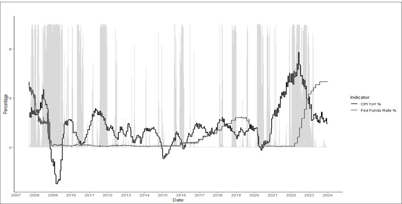
Macroeconomic context and regime probabilities
Source: Author.
In stark contrast, the 2022 market crisis was driven by an inflation shock. The model identifies 2022 as the most persistent period of equity market stress in the sample, but this time, it occurred against a backdrop of soaring inflation that reached multi-decade highs. This forced the Federal Reserve into an entirely different policy posture. Instead of providing accommodation, the central bank was compelled to embark on its most aggressive monetary tightening cycle in decades to restore price stability. This hawkish policy response created a common headwind for both asset classes. Rising interest rates are fundamentally detrimental to both stocks, by increasing the discount rate applied to future earnings, and to bonds, by directly depressing the price of existing fixed-income securities. This common negative driver mechanically forced the stock-bond correlation from negative to strongly positive, thereby dismantling the traditional portfolio hedge. The MSM results, therefore, do not simply identify a statistical anomaly but rather capture the predictable financial market consequences of a fundamental shift in the macroeconomic policy regime.
The practical consequences of this regime shift are severe and cannot be overstated. The drawdown analysis of the 60/40 portfolio, presented in Figure 6, provides a clear illustration of the real-world impact. While the portfolio experienced its deepest single drawdown during the GFC, the recovery was relatively swift, buttressed by the strong performance of its bond allocation. Similarly, the COVID-19 drawdown was sharp but remarkably brief. The 2022 drawdown, however, was both deep and prolonged. The failure of the bond hedge meant a sustained erosion of capital that was unprecedented in the modern era of diversification for the balanced investor.
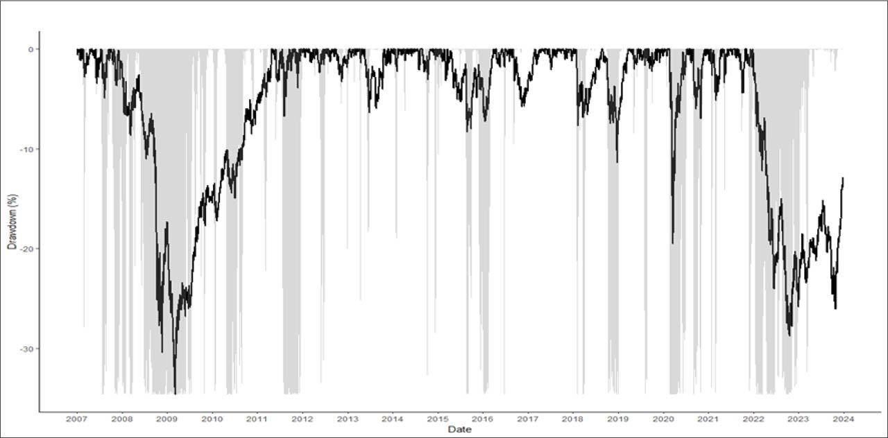
60/40 portfolio drawdowns and crisis regime probabilities
Source: Author.
These findings have implications for both strategic asset allocation and tactical risk management. First, they challenge the foundational assumption of a stable negative correlation that underpins many long-term portfolio construction models. The results suggest that the diversification benefit of government bonds is not a static property but a state-dependent variable, contingent on a low-inflation environment. Risk models that rely on long-term historical correlation matrices would have severely underestimated portfolio risk leading into 2022. Second, the persistence of the “Hedge Failure” regime, which lasted for the better part of two years, suggests that simply waiting for a reversion to the mean is an inadequate strategy. Investors and asset managers must now consider alternative sources of diversification, such as commodities, real assets, or more complex market-neutral strategies that may be more resilient during periods of inflationary stress. The traditional 60/40 portfolio, while historically effective, has been shown to be uniquely vulnerable to the very macroeconomic conditions that emerged in 2022, necessitating a fundamental rethinking of how diversified portfolios should be constructed in the future.
This paper sought to empirically investigate the structural integrity of the traditional stock-bond relationship in the face of the 2022–2023 high-inflation environment. By employing a Markov-Switching model, this study provides rigorous, data-driven evidence that the U.S. stock-bond relationship underwent a fundamental regime change, confirming that the diversification benefits of government bonds are highly state-dependent. The analysis successfully identified two distinct and persistent regimes for both equities and bonds. The key finding is that the nature of the economic shock dictates the prevailing market regime and, consequently, the effectiveness of the portfolio hedge. During the “growth shock” crises of 2008 and 2020, disinflationary pressures allowed for accommodative monetary policy, reinforcing a negative stock-bond correlation and validating the role of bonds as a safe haven. In stark contrast, the “inflation shock” of 2022 compelled an aggressive monetary tightening cycle. This policy response acted as a common headwind for both asset classes, forcing their correlation to turn positive and causing a systemic failure of the classic 60/40 portfolio diversification strategy. The model's results demonstrate that this was not a fleeting anomaly but a persistent regime that dominated the market for the better part of two years, with severe consequences for portfolio drawdowns. The primary limitation of this study is its geographic focus on the U.S. market and its use of a specific set of highly liquid ETFs as asset proxies. While these proxies are standard in the literature, results could vary with different asset choices or in different economic jurisdictions. Furthermore, the analysis centers on a single, albeit highly significant, inflationary event. The findings open several important avenues for future research. A natural extension would be to apply this regime-switching framework to other developed and emerging markets to assess the global prevalence of this phenomenon. Further studies are also warranted to investigate the performance of alternative diversifiers, such as commodities, real assets, inflation-linked securities, and various alternative strategies, within these identified regimes. Such research would be invaluable in helping to construct more resilient portfolios capable of navigating the distinct challenges posed by an inflationary crisis. In sum, this paper's central contribution is its quantitative confirmation that the relationship between stocks and bonds is not a static law of finance but a dynamic one, powerfully shaped by the prevailing macroeconomic regime. For investors and risk managers, this underscores the critical need to move beyond static assumptions and embrace a more dynamic, regime-aware approach to asset allocation.