New Approaches to Complexity via Quantum Graphs

We examine the clique and independent set problems for quantum channels, and we show they are both in QMA(2). Furthermore we prove that the clique problem is QMA(2) -complete and additionally show that, by quantifying over a restricted class of channels, we recover a complete problem for QMA. For deterministic and classical noisy channels, we show that our versions of both the clique and independent set problems are complete for NP and MA, respectively. Our work outlines a hierarchy of decision problems which captures completeness for all four of these important complexity classes and provides evidence for viewing QMA(2) as a natural quantum analogue of NP.

A classical noisy channel N : X → ϒ may be parametrized by a probability transition matrix N = N(y|x), which gives the probability of receiving output y given input x. Given a channel N, the corresponding confusability graph G_N is defined on vertex set X with edges x ~ x′ whenever N(y|x)N(y|x′) ≠ 0, for some y ∈ ϒ, that is, whenever there is non-zero probability that two inputs are mapped to the same output [1]. A set X′ ⊆ X forms an independent set of G_N if x ≁ x′ for all distinct x, x′ ∈ X′, which is if and only if the probability of any pair of distinct x, x′ ∈ X′ being sent to the same output is 0. Similarly, X′ forms a clique of G_N if x ~ x′ for all distinct x, x′ ∈ X′, which is if and only if any pair of distinct elements x, x′ ∈ X′ have a non-zero probability as being received as the same output.

In the quantum setting, classical noisy channels are superseded by quantum channels, represented by completely positive trace-preserving (CPTP) maps Φ : 𝕄_n(ℂ) → 𝕄_m(ℂ). To each such quantum channel, one can associate an operator system 𝒮_Φ ⊆ 𝕄_n, which is constructed as the linear span of all products Ai*AjA_i^*{A_j} for some set of Kraus operators {A_i}_i of Φ. The operator system 𝒮_Φ is independent of the choice of Kraus representation and can be used to generalize the role of confusability graphs to study zero-error capacities of quantum channels. In particular, a collection of orthonormal states |v₁〉, … |v_k〉 can be distinguished from one another with certainty after passing through the channel if and only if |v_i〉〈v_j| is orthogonal to 𝒮_Φ, in which case we say |v₁〉, …, |v_k〉 is an (exact) independent set for Φ or 𝒮_Φ [2]. More generally, one can extend other notions from classical graph theory such as cliques and graph colorings to the setting of operator systems [9,26–28]. In this context, operator systems are often referred to as quantum graphs or non-commutative graphs. For the purposes of this work we use this same terminology, and a quantum graph refers to an operator system 𝒮 inside a matrix algebra 𝕄_n. Below, we discuss how classical graphs can be embedded into the set of quantum graphs, and in Section 1.1.2, we discuss how they can be presented using a quantum circuit.

It is possible to embed classical graphs into the set of quantum graphs in the following way. Starting with an undirected graph G, define an operator system 𝒮_G by taking the span of |i〉〈j| over vertices i and j in G satisfying i = j or ~_G j. Graphs G and H are isomorphic if and only if 𝒮_G and 𝒮_H are unitarily equivalent [28]. Similarly, given a noisy channel N = N(y|x), there are several ways to construct a corresponding quantum channel 𝒮_ΦN which satisfies 𝒮_GN = 𝒮_GN. Generalizations of cliques, independent sets, and colorings to quantum graphs respect this construction, i.e., there is a correspondence between k-cliques, k-independent sets, and k-colorings for G and those for the quantum graph 𝒮_G [24].

Different noisy channels can give rise to the same confusability graph, i.e., the construction N ↦ G_N is not injective. Similarly, in the quantum setting, the construction Φ ↦ 𝒮_Φ is not injective. On the other hand, given any graph G one can construct N satisfying G = G_N with an appropriate choice of transition probabilities N = N(y|x); likewise given any operator system 𝒮 ⊆ 𝕄_n, it is possible to define Φ such that 𝒮_Φ = 𝒮 [24]. Consequently, quantifying over all quantum channels is sufficient to quantify over all quantum graphs, and it is hence well-motivated to consider parameters for quantum graphs at the level of channels.

Recall that, given a graph G, the complement G¯{\bar G} is a graph on the same vertex set where the adjacency relation is defined as i~G¯ji{\~_{\bar G}}j if and only if i ≁_G j. However, there is no generally agreed-upon approach to extending the notion of the graph complement to quantum graphs. One straightforward approach would be to take the orthogonal complement of 𝒮 inside 𝕄_n with respect to the Hilbert-Schmidt inner product, but this will not be an operator system as it fails to contain the identity element, and hence fails to correspond to any channel. One can remedy this by making a correction such as S¯=S+ℂI\overline {\cal S} = {\cal S} + to account for the identity [9]. Unfortunately, this does not extend the graph complement as SG¯≠S¯G{{\cal S}_{\bar G}} \ne {\overline {\cal S} _G}. Another approach allows both operator systems as well as their orthogonal complements to be considered as quantum graphs [27].

Relevant for this work is the fact that there is no straightforward and unique notion of a graph complement for quantum graphs, and consequently, the complexity of decision problems based on cliques and independent sets for quantum graphs cannot be reduced to one another by taking a complement. Indeed, as we discuss in Section 1.5, it is even possible that they have different complexity.

Motivated by the study of non-local games, quantum generalizations of many graph parameters have been found. The existence of k-cliques, k-independent sets, and k-colorings for a classical graph G can be determined by the existence of a perfect classical strategy for a corresponding non-local game. In some cases, quantum strategies for these games can outperform classical strategies, and perfect quantum strategies give rise to quantum cliques and quantum independent sets for classical graphs [29,30]. By considering non-local games where the questions are quantum states, one can also define quantum cliques and quantum independent sets for quantum graphs [31].

It is known that determining the quantum value—or commuting operator value—of a non-local game is an undecidable problem [32–34]. These results can be captured using the non-local games associated to the graph parameters mentioned above, and thus it is undecidable to determine the existence of quantum cliques/quantum independent sets in either classical or quantum graphs [35]. In this work, we take a different perspective and do not consider quantum cliques or quantum independence sets. Instead, we exclusively study the complexity of determining the existence of cliques and independent sets in graphs and quantum graphs.

Problems based on finding cliques, independent sets, or graph colorings are well-studied in classical complexity; they all give rise to NP-complete problems [11]. In these cases, the input to the problem includes an explicit description of the vertices and edges of a graph. Providing an explicit description of a quantum graph raises some challenges: notably quantum graphs are linear subspaces 𝒮 ⊆ 𝕄_n and are thus determined by a basis of operators. As such, given a quantum channel Φ on an n-qubit system, the corresponding quantum graph 𝒮_Φ is a subspace with up to 2²ⁿ dimensions, so specifying it in this way requires a description of an exponentially sized basis. Note that this problem also arises in the classical case, if the graphs in question are seen as arising from a noisy channel on an n-bit input space. For our work, we will instead consider quantum graphs as being determined by an underlying quantum channel Φ, and give a problem instance as a quantum circuit C describing the action of the channel Φ = Φ_C.

The quantum channel 2-clique problem with completeness c and soundness s is the promise problem with yes instances consisting of circuits C such that Φ_C has a (c, 2)-clique, and no instances consisting of circuits for which Φ_C has no (s, 2)-clique. We always assume c ≥ s, and in the cases we consider that there is some probability gap between them. We define the quantum channel 2-independent set problem in a parallel way. In Definition 7, we express these problems more formally and extend them to larger k. These promise problems are written qClique(k)_c,s and qIS(k)_c,s. In this approach, a verifier given a problem instance C may perform computations by running the circuit C in order to implement channel Φ_C, which determines properties of an underlying quantum graph 𝒮_ΦC. The size of a problem instance is then the size of the quantum circuit, which is used to run this computation, rather than the size of an explicit description for the operator system 𝒮_ΦC.

We also consider the restricted problems where the circuits C are only taken from a specific family of quantum circuits 𝒞, which we write as qClique(k, 𝒞)_c,s and qIS(k, 𝒞)_c,s. This allows us to determine hardness results with respect to particular families of channels/quantum circuits such as entanglement-breaking channels and channels that implement partial traces. Importantly, in Section 5, we specify a family of circuits for which these problems are QMA-complete.

In light of the above discussion, we can revisit problems related to cliques and independent sets of classical graphs. More concretely, we consider the input given as a description of a classical circuit which implements a deterministic or probabilistic (noisy) function f on input set X. Note that if X = {0,1}ⁿ, then the confusability graph G_f will be an exponentially sized graph. We then define our decision problems as deciding if the corresponding confusability graph G_f has a clique or independent set of size k. In this approach, the size of the problem instance is related to the runtime needed to compute the adjacency relations in G_f, rather than the size of an explicit description of G_f itself. We also note that our approach differs from graph problems for succinctly presented graphs [36], and to the best of our knowledge has not been studied before from this point of view.

In the case that f is deterministic, the confusability graph consists of a disjoint union of complete subgraphs. In this case, deciding if G_f has a clique of size k = 2 is equivalent to the well-studied collision problem for functions. It asks whether, given some function f : X → ϒ, is there a pair of elements in the domain x, y ∈ X with the same image f (x) = f (y)—a collision. The presumed computational difficulty of this problem on certain classes of functions underlies the security of hash functions, which serve as a primary building block of much of modern cryptography.

More formally, we say a deterministic function f has a k-clique, or a k-independent set, if there exists distinct inputs x₁, …, x_k such that f(x₁) = ⋯ = f(x_k) or f(x₁) ≠ … ≠ f(x_k) respectively. The corresponding decision problems, whose instances are classical circuits describing functions, are denoted Clique(k) and IS(k). We study this case in Section 6.1.

In the case that the underlying function f is probabilistic, i.e., f is a noisy classical channel, the corresponding confusability graph G_f can be more interesting. Indeed, by suitably picking the transition probabilities, it can be observed that any graph on a vertex set V can arise as the confusability graph of some noisy channel f with input set V. In Section 6.2, we study the complexity of deciding the existence of approximate k-cliques and approximate k-independent sets for probabilistic functions. We restate the relevant definitions for the case k = 2 here.

The probabilistic 2-clique problem and the probabilistic 2-independent set problem are the promise problems that consist of deciding the existence of approximate 2-cliques or 2-independent sets, up to some specified promise gap c – s. In Section 6.2, we extend these definitions to larger k and we write pClique(k)_c,s and pIS(k)_c,s for the corresponding promise problems.

First, we devise a new technique to take direct sums of quantum circuits (10). In order to be able to parameterize arbitrary non-unitary channels by means of circuit diagrams, we work with an extended circuit model that appends partial trace and state preparation maps to a basic set of unitary gates. In this way, we extend the universality of a gate set to CPTP maps by means of the Stinespring dilation theorem. At the level of channels, there are a variety of ways to compose the maps to get new ones, but it is not always immediate how that translates to composition at the level of circuits—importantly, whether it is computationally efficient. In our constructions, the way we will combine channels is by means of the direct sum: given two channels Φ₁ and Φ₂ and a probability p, the direct sum is pΦ₁ ⊕ (1 – p)Φ₂, the convex combination of the channels Φ₁ and Φ₂ with orthogonal output spaces. Of course, the circuit model is well-adapted for composition and direct products of maps, but not for sums. To get the wanted superposition of circuits, we might add a qubit in state p|0〉+1−p|1〉\sqrt p |0\rangle + \sqrt {1 - p} |1\rangle , conditionally act by either Φ₁ or Φ₂ based on this qubit, and then measure the added qubit. This, however, has a technical obstruction: conditioning a non-unitary channel can put the number of output qubits in superposition or probabilistic mixture, which is untenable. Instead, we use the fact that the circuits decompose into the basic gates to separate the unitary from the non-unitary gates. Then, the unitary gates act conditionally on the additional modulating qubit as wanted, and the non-unitary gates can be aligned to act the same way for both Φ₁ and Φ₂. In this way, we get a circuit that implements a direct sum of channels of size polynomial (in fact linear) in the size of the circuits describing the original channels. See also Figure 2 for an illustration of this construction. We are optimistic that this direct sum construction might be able to find various other applications in quantum information.

Next, the direct sum construction allows us to port ideas from self-testing over to questions about quantum cliques. The main technical tool we prove to use this technique is Lemma 5. As noted above, the technique takes the direct sum of two channels in order to expand the set of pairs of states on which some property of one of the channels holds. To illustrate how this works, we outline the proof of QMA(2)-hardness of the quantum 2-clique problem (6), which is based on this technique. Given some instance x of a QMA(2) promise problem (ϒ, N), we know that there is some efficiently constructable circuit Φ_x that accepts with high probability on some separable state if x is a yes instance, and with low probability on every separable state if x is a no instance. In the first step, we construct an entanglementbreaking channel Ψ_x that runs this verification, measures, and outputs a pure state if it accepts and a highly mixed state if it rejects (8). Note that this channel acts on one more qubit than Φ_x, which it immediately traces out, in order to have that qubit guarantee orthogonality of any clique. If Φ_x accepts with high probability, then Ψ_x outputs a state close to pure, and thus, the overlap of two input states differing only in the orthogonality qubit will be high. As such, if x is a yes instance, Ψ_x has a clique in the separable states. On the other hand, if Φ_x accepts with low probability, then the output state will be far from pure, resulting in low overlap—as such, a no instance leads to a channel Ψ_x with no cliques among the separable states. The trick however is to lift this property to all the states. To do so, we use the channel Φ₁ constructed in Lemmas 6 and 7, consisting of a direct sum of partial traces on the subregisters we wish to be unentangled. For this channel, we uncover a property reminiscent of self-testing: if states form a near optimal clique, then they must be separable, since partial traces of entangled states are mixed and hence have low overlap. Finally, in the convex combination of Φ₁ and Ψ_x, we find via Lemma 5 that if we weight Φ₁ sufficiently, then the testing for separability overcomes any potential non-separable cliques of Ψ_x, and thus that for a no instance the channel has no cliques. Since the weighting can be chosen to preserve polynomial or constant gaps, this proves the hardness of the 2-clique problem for QMA(2). We believe that this technique is readily extendable to prove other properties of channels; in fact, in Appendix A, we use Φ₁ as well as a channel that guarantees orthogonality among the tensor terms of a separable state to reduce the quantum k-clique problem directly to the 2-clique problem.

It is interesting to note that, though this proof technique is very useful in determining properties of cliques, it seems not to be well-adapted to the study of independent sets. First, Lemma 5 is used to expand collections of states where there is no clique, whereas this would require us to be able to expand collections of states where there is no independent set. A more serious technical obstruction, however, is that where cliques may arise from essentially one source, independent sets arise from two. The overlap of two states is high if they are approximately equal and pure. However, the overlap of two states is low if they are approximately orthogonal or highly mixed. The first corresponds to an approximate version of the independent sets for an operator system, but the second does not. This case of low overlap, which we refer to as a pseudo-independent set, underpins the proofs of hardness of the clique problem, but seems to be an obstruction for the independent set problem. In particular, if we want to guarantee small overlap, it is not required to output orthogonal states—it suffices to output a highly mixed state. Also, high overlap is critical in guaranteeing separability of states by means of Lemma 7. This raises an interesting question: does there exist a channel where the independent sets are separable states? Resolving this would serve to illuminate the complexity of the clique problem greatly.

Finally, our proof of the QMA-completeness of the clique problem for a subclass of the entanglement-breaking channels uses significantly different techniques. The main difficulty lies in showing that this problem actually lies in QMA. This relies on an interesting result of Brandão [43], which shows that the subclass of QMA(2) where the verifier may measure with a Bell measurement—measure each of the factors in the separable state separately, and then classically compute whether or not to accept—lies in QMA. We find that computing the clique value by running the channel and then doing the swap test is in fact a Bell measurement when the channel is entanglement-breaking. Nevertheless, we must still further restrict, because there is another check needed to verify a clique: checking orthogonality of the states. In our proof that the clique problem is in QMA(2), we also do this via the swap test. However, since this swap test is not prefixed by an entanglement-breaking channel, it cannot be evaluated by a Bell measurement. In fact, Harrow and Montanaro [37] show that the swap test cannot even be run by an LOCC measurement, which is a larger class than the Bell measurements. As such, we need a different method to guarantee orthogonality; we work over channels where the output is independent of one of the qubits, i.e., that qubit is immediately traced out. This is the same method as we have used to guarantee existence of an orthogonal clique in the QMA(2)-hard clique problem. As such, the prover need not even send as a proof a clique where the states are orthogonal—the verifier may nevertheless be certain that there exists one. Finally, we note that, unlike the QMA(2)-completeness result, the QMA-completeness result generalizes immediately to the independent set problem as well.

The existence of graph complementation provides a straightforward way to reduce the problems of deciding cliques and independent sets for graphs. This also extends to the versions of these problems introduced in Section 6.

In the quantum setting, our proof technique establishing QMA(2) -hardness for the clique problem qClique (k)_c,s could not readily be extended to the problem qIS (k)_c,s. As discussed in Section 1.1.1, there is no canonical way to take the complement of a quantum graph as there is classically. Instead, several differing approaches have been considered in the literature. Even when one considers the different approaches available, it is not clear how to use these maps on the level of operator systems to obtain an efficient reduction between qClique(k)_c,s and qIS(k)_c,s. Indeed, in an informal sense, it would appear that under any appropriate notion of complementation the complement of a quantum graph can be a significantly more complicated object than the original quantum graph. On the one hand, we know that the quantum independent set problem is contained in QMA(2). On the other hand, it is hard for QMA. However, we feel it is unlikely that there exists a QMA verification circuit for qIS(k)_c,s. This is a similar situation to the pure state version of the QMA-complete consistency of local density matrices problem, which has long been conjectured to be complete for QMA(2) [13]. It is possible that neither of these problems is QMA or QMA(2)-complete, and a reduction from one of the two problems to the other would be enlightening.

Famously, Lovász showed a reduction between the k-coloring problem and the 3-coloring problem in ordinary graphs [44]. In this case, the instances are given using an explicit description of the graph. In Section 6, we introduce new variants of the k-clique and k-independent set problems motivated from the study of noisy channels and confusability graphs. It is straightforward to similarly define a new version of the k-coloring problem. We did not investigate the complexity of this problem but suggest it as worthy area of exploration. Since a coloring on exponentially many vertices cannot be described in polynomial time, it is altogether possible that the class where this coloring problem lives is significantly larger than NP.

In the quantum setting, various approaches to define a k-coloring for a quantum graph have been considered [9,27]. Informally, a k-coloring of a quantum graph 𝒮 ⊆ 𝕄_k consists of a partition of an orthogonal basis for ℂ^k into independent sets. As in the classical case, for an n-qubit quantum channel, this would require specifying a basis for a 2ⁿ dimensional space. It seems unlikely that the corresponding problem could be decided in QMA(2).

There are a variety of decision problems for graphs which can possibly be extended to the quantum setting via a similar approach to the one we use for the clique and independent set problems. We suggest two more here. Firstly, in our problems, the size k of a clique or independent set is a parameter which defines the problem. One can instead consider the value k to be specified along with the circuit description as an input. In the classical case of graphs described by their adjacency matrices, this takes the complexity of finding a clique or independent set from P to NP-hard [11]. One might imagine a similar jump happens in the cases we have considered, from NP, MA, QMA, or QMA(2) to larger classes.

Secondly, one can consider versions of the well-studied graph isomorphism and non-isomorphism problems. In particular, consider a quantum verifier who receives as input a pair of circuits C₁ and C₂ which implement classical or quantum channels Φ₁ and Φ₂. The corresponding promise problems would then be to decide if the quantum graphs 𝒮Φ₁ and 𝒮_Φ1 are approximately isomorphic or far from isomorphic. The quantum analogues of these problems may also provide new approaches to zero-knowledge proof protocols in the quantum setting, since graph isomorphism/non-isomorphism played an important role in early work on zero-knowledge proof systems [45,46]. The area of zeroknowledge proof systems in the quantum setting has seen a flurry of recent advances [13,40,47–49], and it would be interesting if the study of quantum graph isomorphisms can provide new approaches to zero-knowledge in some of these settings.

Another possible area of exploration is Ramsey theory for quantum graphs. Ramsey theory is a branch of mathematics initiated by F. Ramsey which examines the existence of ordered substructures arising in graphs of a sufficient size [50]. Ramsey theory has some interesting connections with computational complexity, such as studying the computational complexity of computing the Ramsey numbers [51]. Several of the motivating themes of Ramsey theory have been explored for quantum graphs [7,52], and it may be worthwhile to explore connections to complexity inspired by these works that incorporate our approaches for presenting quantum graphs as circuits.

While the problems studied here present natural problems which are expressive enough to give complete problems for a variety of well-studied classes, we do not present any concrete applications. It would be interesting to explore how the qClique and qIS problems may have applications in other areas of quantum information theory.

Another potential application may be found using the construction given in Section 4.1.2. This presents a new tool that allows one to take direct sums of quantum circuits as opposed to the more standard tensor product. It would be interesting to see if this has applications in areas such as quantum algorithms or quantum linear algebra.

We use italic capitals H, K, L to represent Hilbert spaces, which we always assume to be finite-dimensional. Given a finite set S, write ℂ^S for the {|S|-dimensional Hilbert space with canonical (computational) basis {|s〉 | s ∈ S}. As a special case, we denote the space of one qubit Q = ℂ^{0,1}. Fix some Hilbert space H. Write H_⊥ for the superspace H + ℂ|⊥〉 where |||⊥〉|| = 1 and 〈⊥|ψ〉 = 0 for all |ψ〉 ∈ H. For any subspace K ⊆ H, write μ_K for the maximally mixed state on K. Write ℬ(H) for the space of linear operators on H, write 𝒫(H) for the space of positive operators, and 𝒟(H) to be the set of density operators (trace 1 positive operators). We use quantum state interchangeably with density operator, specifying to pure quantum states when necessary; we use quantum channel interchangeably with completely positive trace-preserving (CPTP) map.

We denote the set of all bitstrings {0,1}*≔∪n=0∞{0,1}n{\{ 0,1\} ^*}: = \bigcup\nolimits_{n = 0}^\infty {{{\{ 0,1\} }^n}} . Given some x ∈ {0,1}*, write |x| ∈ ℕ for its length. For a function f : ℕ → [0,1], write f : ℕ → (0, 1)_exp to mean that there exist N, k > 0 such that 2^–nk < f (n) < 1 – 2^–nk for all n ≥ N. Write the set of polynomially bounded functions poly = {f : ℕ → ℝ | ∃k, N ≥ 0. f(n) ≤ n^k ∀ n ≥ N}. For a natural number n ∈ ℕ, write [n] := {1,2, …, n}.

A language is a subset L ⊆ {0,1}*. An element x ∈ L is called a yes instance, and an element x ∉ L is called a no instance. A promise problem is a pair (ϒ, N) of disjoint subsets ϒ, N ⊆ {0,1}*. Here, x ∈ ϒ is called a yes instance and x ∈ N is called a no instance, while x ∉ ϒ ∪ N is indeterminate. Promise problems generalize languages in the sense that every language L corresponds to the promise problem (L, L^c). A complexity class is a collection of languages or promise problems.

A function f : {0,1}* → {0,1}* is computable in time T(n) if there exists a Turing machine M that, on input x, outputs M(x) = f(x) in T(|x|) steps. We say f is polynomial-time computable if there exists a polynomial p : ℕ → ℕ such that f is computable in time p (n).

A language L₁ is polynomial-time Karp-reducible to another language L₂ if there exists a polynomial-time computable function f such that x ∈ L₁ iff f(x) ∈ L₂. For promise problems, a similar definition holds, the only difference being that the function must map no instances to no instances as well. Given a complexity class C, L is C-hard (under polynomial-time Karp reductions) if every element of C is polynomial-time Karp reducible to L. L is C-complete if additionally L ∈ C.

In its usual usage, the circuit model of quantum computation is used to describe unitary channels. To describe unitaries, we fix a (finite) universal gate set S ∈ 𝒰_n0(ℂ)—in this work, we do not need to specify the choice of gate set, but one can, for example, always assume that it is the Clifford+ T gate set {CNOT, H, T}. We can approximate any unitary to arbitrary precision by a composition of finitely many tensors of the basic gates.

In order to describe all quantum channels, we need to add two non-unitary operations, that change the number of qubits, to the basic gate set:

• The partial trace on one qubit Tr : ℬ(ℂ²) → ℂ;

• State preparation of one qubit in the computational basis ℂ → ℬ(ℂ²), λ ↦ λ|0〉〈0|.

Due to the Stinespring dilation theorem, the augmented gate set S ∪ {Tr, |0〉〈0|} can approximate any quantum channel to arbitrary precision. Stinespring dilation also guarantees that the circuit can be expressed in a canonical form where qubit preparation happens first, followed by unitary gates, followed by partial traces. In fact, given a circuit description, it can be taken to this canonical form efficiently simply by sliding the state preparations backwards and the partial traces forwards. As such, we will assume that the circuits are always in this form.

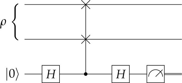
Note that POVM measurements can in particular be realized in this model. For example, measurement of a qubit in the computational basis can be realized by the following circuit:

Other measurements can be realized similarly—diagonalizing for PVMs or using Naimark’s theorem for general POVMs—although the circuit representations may consist of many gates.

For the computational problems we consider, the instances take the form of circuit diagrams describing some quantum channel. It is perhaps simplest from the theory standpoint to present the diagrams as pictures, but it is wholly equivalent to represent the circuits as an encoding of the diagram as a bitstring, which is more natural from a computational standpoint. For a circuit diagram C, write Φ_C for its implementation as a quantum channel. We take the length of the circuit |C| = in(C) + out(C) + gates(C), the sum of the number of input qubits, the number of output qubits, and the number of gates. Note that it is possible to choose an encoding as a bitstring whose length is polynomial in the circuit length described above, and vice versa.

We can also treat classical circuits in a similar way. Here, circuits describe not channels but functions f : {0,1}^m → {0,1}ⁿ. But, as in the quantum case, we can choose a finite universal gate set, for example, {NAND}. Given a classical circuit diagram C, write f_C for the function it represents and |C| = in(C) + out(C) + gates(C) for the circuit size.

There are a variety of natural distance measures between quantum states; we use three: the Euclidean norm, the trace norm, and the Frobenius (or Hilbert-Schmidt) norm. The Euclidean distance is only defined on pure states and is simply the natural norm induced by the inner product on the Hilbert space ‖|ψ〉‖=〈ψ∣ψ〉|\psi \rangle = \sqrt {\langle \psi \mid \psi \rangle } . The trace norm is defined for all A ∈ ℬ(H) as ‖A‖Tr=12Tr[A†A]A{_{{\mathop{\rm Tr}\nolimits} }} = {1 \over 2}{\mathop{\rm Tr}\nolimits} [\sqrt {{A^\dag }A} ]; and the Frobenius norm is defined similarly as ‖A‖2=Tr[ A†A ]A{_2} = \sqrt {{\mathop{\rm Tr}\nolimits} \left[ {{A^\dag }A} \right]} . The following simple lemma relates the metrics that these norms induce on the pure states. We use this extensively and without mention.

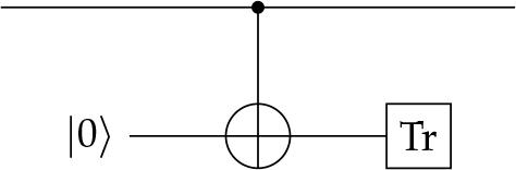
The swap test, first introduced in [53], provides a computationally efficient way to project on the symmetric subspace of a tensor product Hilbert space— the +1 eigenspace of the swap operator that exchanges the two tensor terms. The swap test proceeds on a state ρ ∈ 𝒟 (H ⊗ H) as follows:

• Prepare an auxiliary qubit in the state |+〉.

• Act with the swap operator on ρ conditionally on the auxiliary qubit.

• Measure the auxiliary qubit in the Hadamard basis. Accept if the measurement result is 0 and reject if not. The swap test is illustrated as a quantum circuit in Figure 1.

Figure 1.

Quantum circuit representation of the swap test.

Let Π_H : H ⊗ H → H ⊗ H be the projector onto the symmetric subspace. Then, the swap test implements the channel ρ↦ΠHρΠH⊗|0〉〈0|+(I−ΠH)ρ(I−ΠH)⊗|1〉〈1|\rho \mapsto {\Pi _H}\rho {\Pi _H} \otimes |0\rangle \langle 0| + \left( { - {\Pi _H}} \right)\rho \left( { - {\Pi _H}} \right) \otimes |1\rangle \langle 1|. It’s also useful to note that, if ρ is a separable state ρ = ρ₁ ⊗ ρ₂, then the probability of the swap test accepting is 12+12Tr[ ρ1ρ2 ]{1 \over 2} + {1 \over 2}{\mathop{\rm Tr}\nolimits} \left[ {{\rho _1}{\rho _2}} \right].

In this section, we introduce and study the complexity of the promise problem of deciding the existence of an approximate independent set/clique for a quantum channel, given as a circuit.

The main results of this section are to show that all of the above problems are in QMA(2) for c, s : ℕ → (0,1)_exp with polynomial gap, and to show that the quantum 2-clique problem for some class of channels is in fact QMA(2)- hard. First, we recall the formal definition of QMA(2).

We know that whenever c, s : ℕ → (0,1)_exp and have polynomial gap, then QMA(2)c,s=QMA(2)23,13≕ QMA(2){\rm{QMA}}{(2)_{c,s}} = {\rm{QMA}}{(2)_{{2 \over 3},{1 \over 3}}} = :{\rm{ QMA(2)}}, as for MA and QMA. Due to [37], we also know that QMA(P) = QMA(2) for P : ℕ → ℕ any polynomial number of provers.

Next, we want to show that the quantum clique problem is in fact QMA(2)-hard as well. In fact, we show the stronger property that a subclass of all channels achieves this hardness. First, we introduce this subclass.

Write 𝒞_EB for the set of quantum circuits representing entanglement-breaking channels. Write 𝒞_Tr for the collection of circuits that are partial traces on some of the qubits.

The name entanglement-breaking for these maps arises since, if Φ is entanglement-breaking, then the output state of 𝕀 ⊗ Φ is always separable. These are the only maps with the property. For more on entanglement-breaking channels, see for example [54,55].

The circuits we are interested in combine the above two restricted classes of channels by means of a direct sum. At the level of channels, we mean to use channels of the form pΦ_Tr ⊕ (1 — p)Φ_EB To do so, we need a way to form the direct sum of two quantum circuits.

Note that the state p|0〉+1−p|1〉\sqrt p |0\rangle + \sqrt {1 - p} |1\rangle cannot be generated exactly by finitely many gates from the gate set for all but countably many values of p. However, for any p, polynomially many gates (in the circuit sizes) can be used to construct an exponentially good approximation to the state, which we use to keep the circuits of reasonable length. See also Figure 2 for an example of the implementation of the above definition.

Figure 2.

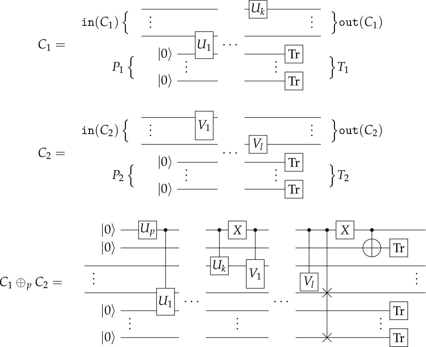
Representation of the construction of the circuit C₁ ⊕_p C₂ from the circuits C₁ and C₂ in canonical form, with out(C₂) < out(C₁). U_p is a unitary that implements the map |0〉↦p|0〉+1−p|1〉|0\rangle \mapsto \sqrt p |0\rangle + \sqrt {1 - p} |1\rangle to good approximation.

Using the natural identification, for m > n, of Q^⊗m ⊕ Q^⊗n with the subspace |0〉⊗Q⊗m+|1〉⊗Q⊗n⊗|0m−n〉⊆Q⊗(m+1)|0\rangle \otimes {Q^{ \otimes m}} + |1\rangle \otimes {Q^{ \otimes n}} \otimes \left| {{0^{m - n}}} \right\rangle \subseteq {Q^{ \otimes (m + 1)}}, we see that ΦC1⊕pC2=pΦC1⊕(1−p)ΦC2{\Phi _{{C_1} \oplus p}}{C_2} = p{\Phi _{{C_1}}} \oplus (1 - p){\Phi _{{C_2}}}. Note also that, by the above definition |C₁ ⊕_p C₂| = O (|C₁| + |C₂|).

To prove this theorem, we develop a technique to take a channel whose cliques have certain properties with respect to a set of states, and combine it with another channel in order to enlarge the set of states on which those properties hold. This is inspired by self-testing techniques, such as Lemma 5.5 of [40].