
1. Introduction
Shor’s algorithm [1,2] for factoring integers has become one of the examples of a practically relevant problem, which is hard for classical computers yet amenable for quantum processors. The implication of the integer factorization problem to the widely adopted cryptographic schemes, such as the RSA cryptosystem [3], is a clear motivation for studying its practical complexity within both the classical and quantum approaches [4,5]. Proof-of-concept experimental factoring of 15, 21, and 35 has been demonstrated on superconducting [6], trapped ion [7], and photonic [8-10] quantum computers. However, the implementation of Shor’s algorithm for breaking of actually employed cryptosystems requires resources, which seem to be far beyond the capabilities of existing and upcoming generations of quantum computing devices. For example, in order to factor a 2048-bit RSA integer (i.e., an integer N = pq where p, q are distinct primes), one would need 8 hours using 20 million noisy qubits [11]. Recently, this requirement has been updated to less than a week using less than a million noisy qubits [12].
While current quantum computers are not yet capable of running Shor’s algorithm in a regime that provides a quantum advantage, various approaches are being developed to implement factorization with fewer resources [13–15] or even with currently available noisy intermediate-scale quantum (NISQ) devices [16–18]. One of the proposed methods is the use of the variational quantum factorization (VQF), which has been applied to factorize 41-, 12-, and 13-bit integers on three, four, and five superconducting qubit systems, respectively [19]. The approach incorporates classical preprocessing that yields variable quantum resource requirements across different integers, with some cases achieving particularly significant qubit reductions. The recent paper [20] utilizes an IBM superconducting processor to factorize an 8-bit integer (253) using 9 qubits, without the need for classical preprocessing. This is achieved by applying the variational quantum eigensolver (VQE), which minimizes (N – pq)2 to obtain the desired factorization. Additionally, [20] also presents a simulation of the factorization of up to 20-bit integers using up to 27 qubits.
Another approach, proposed in [21], combines Schnorr’s factorization method [22] with the quantum approximate optimization algorithm (QAOA) [23,24], which can be efficiently implemented on NISQ devices [25–28]. The seminal work [21] demonstrated the factorization of a 48-bit integer on 10 trapped ion qubits, describing the solution to a single subproblem using a quantum-classical hybrid quantum QAOA approach. However, as it has been shown [29,30] such an approach encounters a number of pitfalls coming from both classical and quantum domains. In particular, it has been observed [29] that demonstrating this subproblem solution does not equate to full factorization. Building on this, [31] investigated factorizing the same 43-bit integer using a digitized-counterdiabatic quantum algorithm. Their results demonstrated an improved success probability for one Hamiltonian identified in [21], though full factorization was not achieved.
In this study, we show that certain challenges associated with the QAOA-based factorization process can be addressed by switching to a fixed-point variant of QAOA (fpQAOA) [32]. While it became a routine to run QAOA with classical optimization of expectation values with respect to the parameters, such an approach suffers from the problem of global optimization and statistical fluctuations. To our knowledge, the alternative idea to exploit so-called universal angles (parameters) in the QAOA has been presented for the first time in [33]. We follow the latter approach so that in our fixed-point version of QAOA [32] we use fixed optimal parameters from the corresponding training set of tasks, normalize it (i.e., Hamiltonians), and then search for angles providing the maximum minimal increase in the probability of a correct answer, whereas the Max-Min problem is solved via evolution optimization. This allows us to solve reliably the closest vector problem (CVP), which lies in the basis of Schnorr’s algorithm, with the use of the quantum device. Within this approach, we demonstrate experimental factoring of the number 1591 = 37 × 43 using 6 qubits with a trapped ion quantum processor; see Table 1. We also present simulation results for 74425657 = 9521 × 7817 and 35183361263263 = 4194191 × 8388593 with 10 and 15 qubits, correspondingly. These results demonstrate an improvement in the required resources, compared to the simulation results presented in [20], which factored a 20-bit integer using 27 qubits. Although we expect that one of the difficulties in the realization of the QAOA-based factoring is resolved, this approach still requires further scalability studies.
Table 1.
Comparison of the main results of the NISQ factoring in the current work with previous studies.
| Method | N | Qubits | Integer-specific | Full factoring |
|---|---|---|---|---|
| Schnorr + QAOA [21] | 48-bit | 10 trapped-ion | no | no1 |
| Schnorr + DCQA [31] | 48-bit | 10 trapped-ion | no | no1 |
| VQF [19] | 41-bit | 3 superconducting | yes2 | yes |
| VQE [20] | 8-bit | 9 superconducting | no | yes |
| Schnorr + fpQAOA (current work) | 11-bit | 6 trapped-ion | no | yes |
2. Fixed-Point QAOA-Based Factoring
Here we describe the main principles of the considered algorithm, Figure 1 shows the scheme of factoring, and the detailed description is presented in the Supplementary Materials. The crucial component of Schnorr’s factoring algorithm is the search for smooth relation pairs of integers, so-called sr-pairs. The definition of sr-pair is based on the factor base Pn: the set {pi}i=0,…,n of the first n primes together with – 1 (p0 = – 1, p1 = 2, p2 = 3,…). A pair of integers (u, v) is called an sr-pair (for fixed Pn and an integer N) if u and u – vN have prime factors only from Pn. Note that the size of the factor base n is the most important hyperparameter of the algorithm (depending on the size of the factorized number N) and is also equal to the number of qubits of the quantum part.
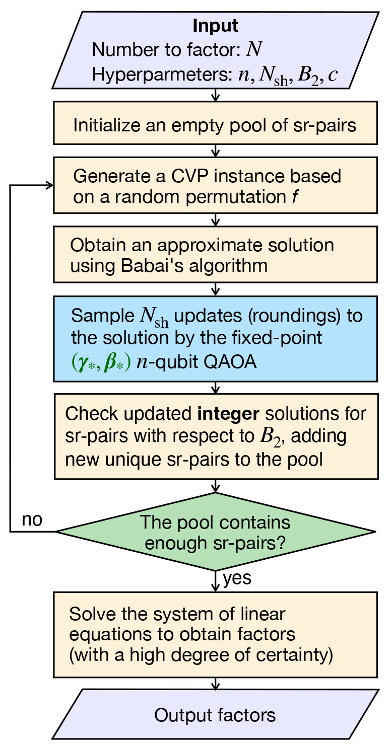
Figure 1.
General scheme of the QAOA-based Schnorr factoring algorithm.
As soon as we have a sufficient number of such pairs, which is larger than the size of the factoring base (hyperparameter of the algorithm), we can form a system of linear equations that appears to be degenerate and always has a solution. This solution, by a classical Fermat’s method (see, e.g., [34]), provides a factorization with a high probability.
The problem of sr-pairs search can be reduced to the closest vector problem on a lattice: one needs to find the linear combination of vectors with integer coefficients closest to the target vector
with integer coefficients closest to the target vectorHere f(i) is the random permutation of the first n natural numbers, c is the smoothness hyperparameter, and N is the integer to factorize. The closer the found solution to the desired vector, the greater the chance of obtaining an sr-pair.
Schnorr’s method relies on solving the CVP with the classic approximate Babai’s algorithm [35] with LLL-reduction (Lenstra–Lenstra–Lovász) [36]. As this algorithm gives only an approximate real-valued solution, in the original paper by Schnorr it was rounded to the closest integer value at the last step. The idea behind the recent proposal [21] is to choose the rounding side for each variable to find the closest integer-valued solution, which in turn directly reduces to a quadratic unconstrained binary optimization (QUBO) problem. The example of the rounding refinement is presented in Figure 2. Such class of problems is amenable to solving with QAOA
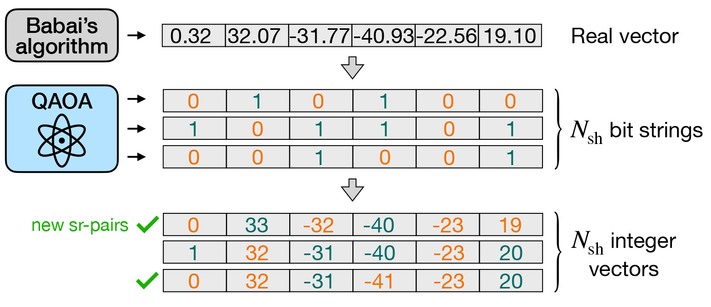
Figure 2.
The example of the rounding refinement in the QAOA-based Schnorr factoring algorithm.
QAOA is based on the trotterization of the adiabatic evolution of the following form:
where β = {β[j]} and γ = {γ[j]} are circuit parameters (angles), hyperparameter p is the number of layers, | + ⟩ is the +1 eigenstate of σx Pauli matrix, is the mixing Hamiltonian (here is σx acting on k-th qubit), and HP is the problem Hamiltonian, which in most cases directly encodes the Ising form of a QUBO problem to be solved.The most common approach to QAOA is to classically optimize the expectation value E (β, γ) = 〈β, γ | Hp | β, γ〉 being estimated by the set of measurements (shots) on a quantum processor (see, e.g., Refs. [37–39]). In contrast, in the seminal QAOA paper [23] relies on searching optimal angles utilizing the efficient exact classical calculation of E (which was presented for Max-Cut problems on 3-regular graphs [23]) followed by sampling on a quantum processor. We have used an alternative approach based on the empirical hypothesis of close optimal angles for different instances of the same problem type [33,40,41].
To find fixed QAOA parameters, we use the training set consisting of 100 QUBO subproblems arised during factoring N = 48567227 on n = 10 qubits. As optimal QAOA problem angles γ scale together with QUBO coefficients, we normalize every QUBO coefficient matrix by its maximal value [32]. The ratio Pq / Pc of the probability Pq to measure the optimal (minimal) answer to its classical random sampling counterpart Pc was used as an optimization metric, and its minimum over the training set was maximized using random mutations optimization algorithm [42,43]. To minimize the quantum circuit depth, we use just a single layer of QAOA (p = 1), which significantly increases robustness of the quantum part of the algorithm. The quantum circuit for a single layer of QAOA used in the algorithm has the form presented in Figure 3, and Figure 4 demonstrates the scheme of the fpQAOA.
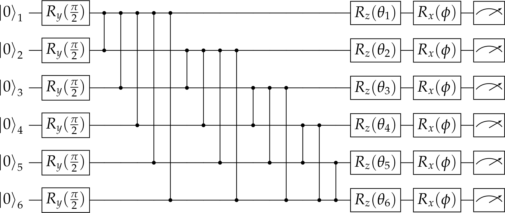
Figure 3.
Architecture of the executed quantum circuits in fixed-point-QAOA algorithm. Each pair of connected black circles corresponds to ZZ (χij) gate acting on i-th and j-th qubits, where for each involved qubit pair χij is unique. Angles θi in Rz (θi) gates are also different for each i-th qubit in each circuit. β in Rx (φ) is equal to 2.64. For each of the 9 executed circuits parameters of these gates are given in Table 5 of Supplementary Materials.
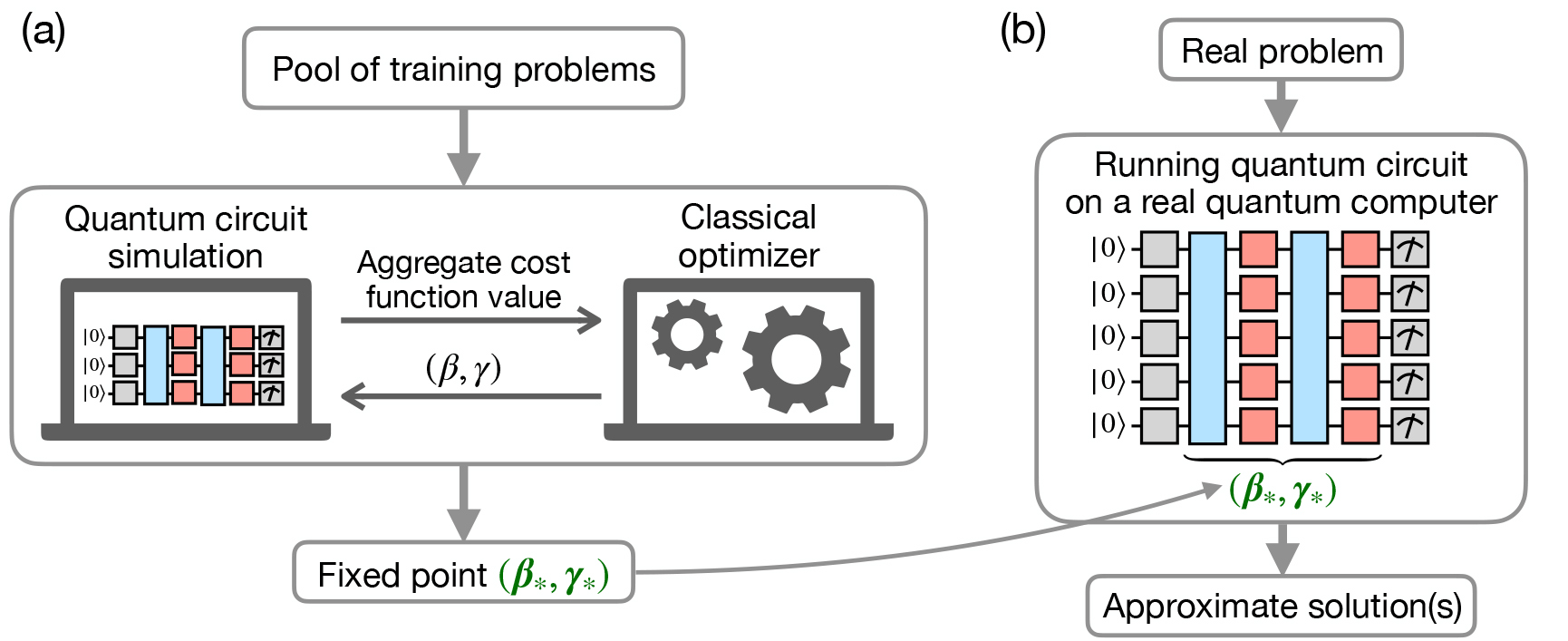
Figure 4.
Scheme of the fixed-parameters QAOA algorithm: (a) training—search for fixed parameters; (b) using for real problems.
The resulting single-layer QAOA parameters used in the factorization are γ1 := γ* = 2.64 and β1 := β* = 0.33. The fixed-parameters approach allows avoiding the classical-quantum hybrid optimization procedure and fits well with the demands of Schnorr’s method: one does not need to obtain the exact or suboptimal solution of CVP, but sample solutions close to the target vector to increase the probability of forming a set of sr-pairs.
In the classical part of the algorithm, we directly follow Refs. [21] and [29]. We use the main factor base of the size B1 = 6 (which is equal to the number of qubits), the relaxed factor base size for sr-pairs verification is B2 = 11, the rounding parameter of lattice/target formation procedure is c = 1.5, and the parameter of LLL-reduction is δ = 0.75. For each lattice (which is formed by a random permutation of the diagonal), we conduct 5 measurements (shots) of each circuit. Due to a strongly stochastic nature of the algorithm the required number of circuits varies. The details of a single run of the factorization algorithm including the exact form of the circuit and corresponding parameters are provided in the Supplemental Material.
3. Experimental Setup
Experimental demonstration of the algorithm was performed with a quantum processor based on a chain of ten ultracold 171 Yb+ ions in a linear Paul trap. Its characteristics are summarized in Table 2. Qubits are encoded in states |0〉 = 2S1/2 (F = 0, mF = 0) and |1〉 = 2D3/2 (F = 2, mF = 0), coupled by an optical E2 transition at wavelength λ = 435.5 nm. While the setup supports usage of all five Zeeman sublevels of the upper state for the information encoding (i.e., we have the qudit processor [44]); in this work we have used the processor in the qubit regime.
Table 2.
Parameters of the experimental setup.
| Parameter | Value |
|---|---|
| Number of qubits | 10 |
| Single-qubit gate fidelity | 99.946(6)% |
| Two-qubit gate fidelity1 | 96.3(3)% |
| 30(2) ms | |
| Connectivity | Full |
| Single-qubit gate duration | 20 μs |
| Two-qubit gate duration | 1.14 ms |
| Secular frequencies (ωx, ωy, ωz) | 2π × (3.7, 3.6, 0.13) MHz |
Before each experimental shot ions are Doppler cooled to the temperatures of approximately 1.5 mK, which is followed by the sideband-cooling of all radial motional modes close to the ground state and initialization to the |0〉 state by optical pumping [44]. On the next stage the target native gates sequence is being implemented. In our system single-qubit native gates are Rϕ(θ) = exp(–iσϕθ/2) and Rz(θ) = exp(iθ|1〉 〈 1|), where σϕ = cosϕσx + sin ϕσy, and ϕ, θ — arbitrary angles. The first operation is performed by applying a laser pulse, resonant to the |0〉 → | 1〉 transition. In this case ϕ is determined by the relative phase of the laser field and the qubit, while θ is determined by the pulse duration. The Rz (θ) is a virtual gate [45] and is performed by shifting phases of all successive laser pulses applied to this ion. A native two-qubit operation for this system is a Mølmer-Sørensen gate [46-49] Rxx (2χ) ≡ XX(χ) = exp(–iχσx ⊗ σx). This gate is implemented by illuminating a target pair of ions with a bichromatic laser fields, coupling their electronic states with a collective motional degrees of freedom (in our case we use radial motional modes). These common motional modes serve as mediator, coupling both qubits. The laser fields are amplitude-modulated to decouple all electronic degrees of freedom from motional ones at the end of the gate and reduce sensitivity of the operation to the experimental parameters [50]. The processor supports XX (χ) gates with arbitrary χ and all-to-all connectivity. We also include Rzz (2χ) ≡ ZZ(χ) = exp(–iχσz ⊗ σz) gate in the list of supported operations, which is automatically hardware-efficiently transpiled as ZZ(χ) = (Ry (π/2) ⊗ Ry (π/2))XX(χ)(Ry (–π/2) ⊗ Ry (–π/2)) in the processor. At the end of each experimental shot the quantum register readout is performed using electron-shelving technique on the |2S1/2) → |2P1/2) transition at 369 nm [44, 51]. Ions fluorescence in this process is collected with a high numeric aperture lens and is sent via an array of multimode fibers to the multichannel photomultiplier tube.
Fidelities of the single-qubit and two-qubit operations are 99.946(6)% and 96.3(3)%, which are measured using randomized benchmarking [52], and parity oscillations observation [53], correspondingly. The qubits coherence time ms was extracted from decay of Ramsey fringes contrast with increasing delay between π/2 pulses. To reduce cross-talk during single-qubit operations all Rϕ (θ) gates in the circuits are substituted with their composite analogues using SK1 scheme [54]. Particularly, two 2π rotations around specific axes are added after each singlequbit gate, which are known to suppress both cross-talks and rotation angle fluctuations.
More details on the experimental setup can be found in [44,55].
4. Experimental Results
In the experiment, we use Schnorr’s approach assisted with the fixed-angles QAOA to factorize number 1591 = 37 × 43 using 6 qubits.
In a single sample run of the experiment (for details, see Supplemental Material), B2 + 1 sr-pairs required to deterministically factorize the number were found in 43 steps (shots) using 9 different quantum circuits (each circuit repeated 5 times followed by the next circuit). However, in this particular sample run the first 39 shots appeared to be already sufficient to factorize the number. We have compared the average speed of collecting unique sr-pairs in three cases: (i) random sampling; (ii) experimentally obtained samples; (iii) samples obtained with noiseless emulator (see Figure 5(a)). The figure demonstrates the advantage of the quantum processor sampling results over the random sampling. However, the presence of the noise in the system decreases the efficiency of the method in comparison with a noiseless emulator. To illustrate the level of the noise in the quantum processor we also measured the output states probability distributions for several used circuits with better averaging and compared it with results expected in the absence of errors (for details, see Supplemental Material).
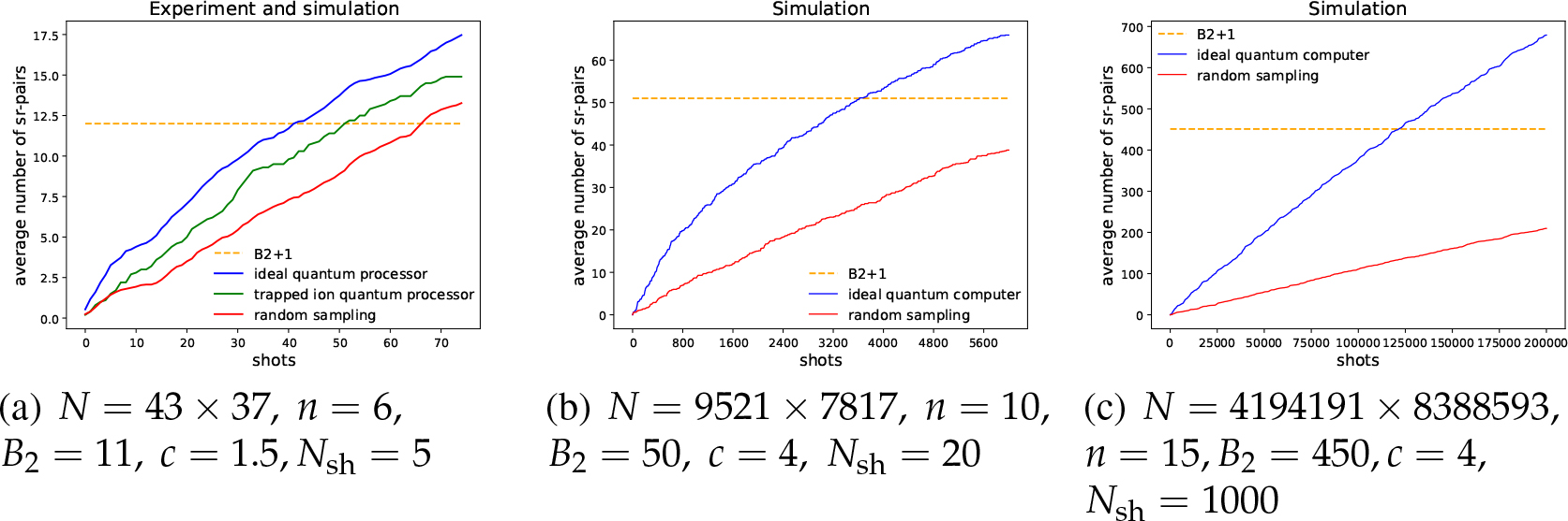
Figure 5.
A comparison of sr-pairs collection rates between cases where QUBO-subproblems samples are generated with a random sampling (red lines), a noiseless quantum emulator (blue), and a real trapped-ion quantum processor (green) for different number of qubits. The left sub-figure shows both experimental (averaged over 10 runs) and simulation data (averaged over 30 runs), while other figures contain only simulation results (averaged over 10 trajectories). Here N stands for the factorized number, n is for the number of qubits, and Nsh is for the number of shots per circuit. The dashed horizontal line shows a B2 + 1 sr-pairs threshold which guarantees the factorization.
In this experiment we chose to use 6 qubits as a trade-off between the problem size and quantum circuits fidelity. Numeric simulations show that the expected advantage over random sampling in QUBO-subproblems increases with the growth of qubits number and magnitude of a number to factorize (e.g., see Figure 5). At the same time as the number of two-qubit operations in each circuit is equal to n(n – 1)/2, where n is the number of qubits, the quantum sampling fidelity decreases with larger n. In our experiments n = 6 was the smallest number of qubits, where the advantage over random sampling was observed experimentally despite the better sampling fidelity at n < 6.
A number of shots per circuit was chosen using numerical simulations. It was set to be sufficient to find enough sr-pairs, keeping the total number of shots minimal.
5. Scalability Analysis
The initial complexity estimates presented in Schnorr’s work [22] did not lead to practical results for factoring large numbers; however, the effectiveness of the method has still neither been proven nor strictly disproved. Based on Refs. [29,30,56,57] and own numerical experiments, the following difficulty can be noted: the probability that estimates obtaining an sr-pair by suboptimal solutions of CVP problem (obtained by classical or quantum methods) does not directly lead to the probability of obtaining a set of unique sr-pairs needed for the factorization. Further, we present a brief empirical analysis of scalability of the presented method. We use the number of measurement shots as a proxy for computational cost, as we adopt an exponential complexity model that ignores polynomial factors from quantum circuit depth (though this can be extended with circuit-level details). Figure 6 shows the logarithmic shot count versus the bit-length nb of the factored integers.
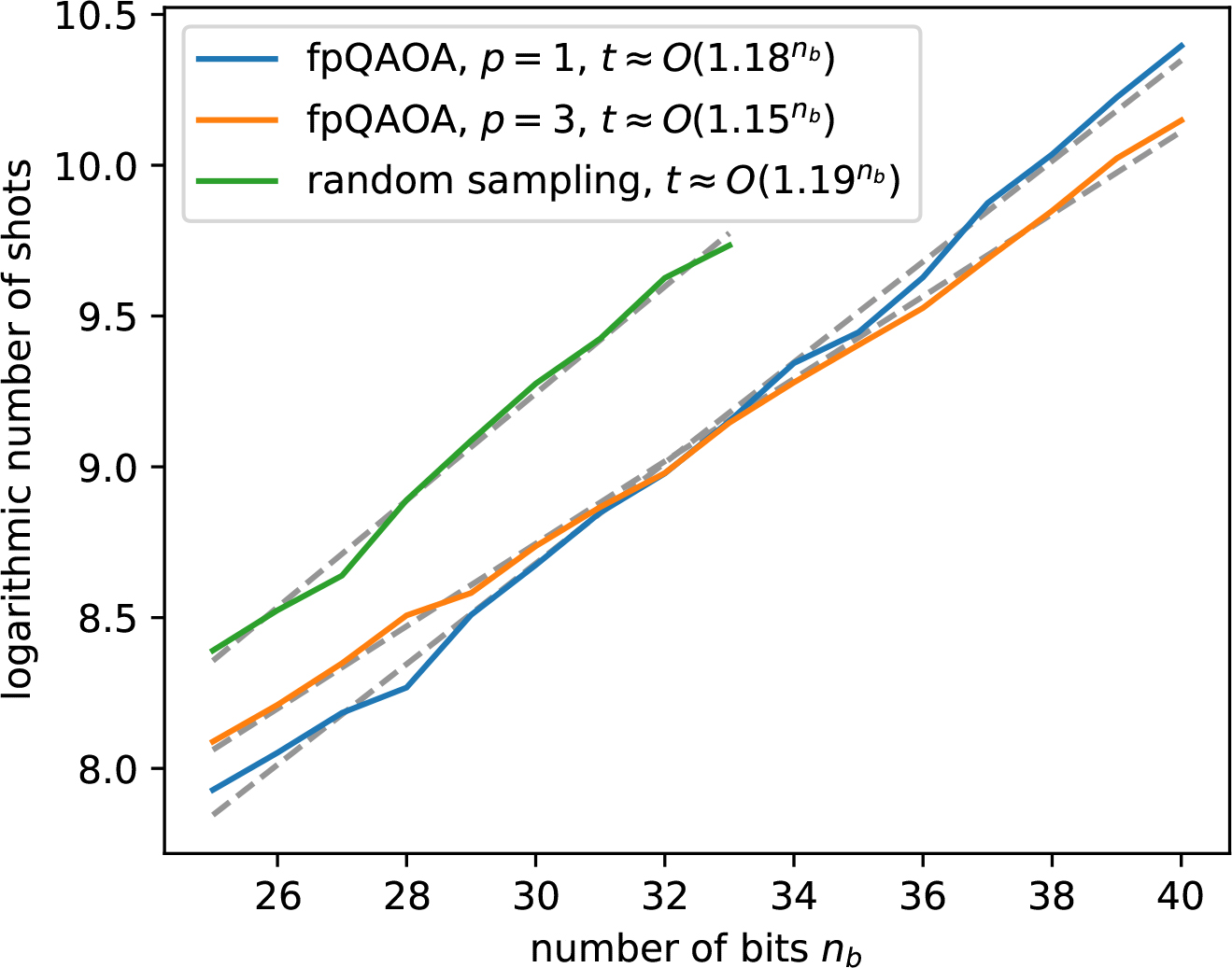
Figure 6.
Dependency of computational complexity (number of shots) on the number of bits.
For fpQAOA-based factoring, we trained on 50 QUBO instances generated from random 24-bit integers using n = 10 (where n denotes the lattice size and the number of qubits). Since optimal parameter selection for n remains an open problem, we performed a grid search to determine the best n for each bit-length and algorithm variant; optimal values of n are presented in Table 3.
Table 3.
Optimal n for different bit-lengths and QUBO-solving methods.
| method / nb | 25 | 26 | 27 | 28 | 29 | 30 | 31 | 32 | 33 | 34 | 35 | 36 | 37 | 38 | 39 | 40 |
| fpQAOA, p = 1 | 11 | 10 | 11 | 11 | 11 | 12 | 12 | 11 | 12 | 12 | 12 | 13 | 12 | 14 | 12 | 13 |
| fpQAOA, p = 3 | 12 | 14 | 12 | 14 | 15 | 14 | 14 | 14 | 14 | 14 | 15 | 15 | 15 | 15 | 16 | 16 |
| random sampling | 9 | 9 | 9 | 9 | 9 | 10 | 10 | 10 | 10 |
Numerical experiments on 25–40-bit integers reveal approximately exponential scaling within the tested range (Figure 6)—consistent with other NISQ-era quantum heuristics [58,59]. Results indicate that the shot count scales roughly as O(1.15nb) for p = 3 QAOA, even for such a low depth outperforming random sampling (m ≈ 1.19) and classical brute-force (m ≈ 1.414). While this suggests a quantum advantage for mid-scale factoring, we emphasize that this model is provisional—its validity at cryptographic scales (e.g., nb > 100) remains untested (the true complexity could be strictly better or worse than this exponential estimate depending on the interaction between Schnorr’s lattice reduction and quantum optimization dynamics). We also want to note that for exponential scaling O(mnb), values like m ≈ 1.02 (enabling classical record 829-bit factoring in 107 shots) may yield practical utility despite asymptotic limitations, as the base m dominates at intermediate scales.
The improvement of complexity of the presented method can possibly be achieved by hyperparameter optimization, increasing the depth p, dynamic p-scaling via Fourier encoding [38], and the enlargement of search spaces beyond single steps from classical approximations. We also emphasize that the quantum advantage should be verified against classical QUBO-solving methods more sophisticated than random sampling.
6. Conclusion and Outlook
We have considered the Schnorr factoring scheme, where following the idea from [21], we adopt the QAOA method at the last step of Babai’s algorithm. However, for the first time we used a fixed-point feature of QAOA [32,33] for the factoring problem and were able to factor a specific integer. To the best of our knowledge, it is the first successful experimental factoring of a particular integer with fixed-point QAOA-assisted Schnorr approach, whereas previously it was only experimentally presented how to obtain some sr-pairs for this task using quantum computers.
To confirm both the overall scheme and the fixed-point approach, we experimentally factor 1591 = 37 × 43 using 6 qubits of the 10-qubit trapped-ion processor. Thus, this work provides the first complete implementation of quantum-enhanced Schnorr’s lattice-based factorization, filling a critical development gap among alternative quantum factoring methods. The fixed-angle QAOA approach enables scalable factoring of general integers, with simulations up to 45 bits on 15 qubits suggesting practical utility for near-term NISQ experiments and benchmarks.
For further research we leave the questions of the algorithm’s efficiency and thorough comparison with classical methods, as well as a more detailed investigation of the quantum processor noise influence.
Note added. After completion of this work, we became aware of [59], which also suggests using fixed-point QAOA in the same context. Authors have presented an alternative approach of fixed angles search and scaling, and conducted a thorough numerical analysis of QAOA-augmented refinement of CVP problem. In contrast, in our work we consider the complete factorization algorithm and its experimental trapped-ion implementation.
Acknowledgments
The authors would like to thank B. I. Bantysh for insightful comments and anonymous referees for their constructive feedback.
Notes
[4] Contributed by Author Contributions
A.Yu.Ch. implemented the fpQAOA subroutine. S.V.G. implemented classical subparts of the algorithm. A.S.N. adapted quantum part of the algorithm for execution on the trapped-ion processor. I.V.Z and A.S.B. performed the experiment. I.V.Z., A.S.B., I.A.S., K.P.G., N.V.S., and A.E.K. built, optimized and operated the quantum processor. E.O.K., A.S.N., and I.V.Z, conducted a theoretical analysis of the experimental results. E.O.K. created the visual illustrations for the article. K.Yu.Kh., A.K.F., I.A.S., and N.N.K. supervised the project. Writing—original draft, all authors have contributed equally to this task. Writing—review and editing, all authors have contributed equally to this task. All authors have read and agreed to the published version of the manuscript.
[5] Conflicts of interest Conflicts of Interest Statement
The authors declare no conflicts of interest.
[6] Data Availability Statement
The data that support the findings of this study are available from the corresponding author upon reasonable request.
Supplemental Materials
In this supplemental section we provide the details of a single run of the factoring algorithm. Let’s consider the first random permutation (1, 3, 2, 5, 6, 4) used in the algorithm. The corresponding CVP is defined by the lattice
and the target vectorThe approximate solution given by Babai’s algorithm based on LLL-reduction is
all elements were rounded up to the nearest integer. The corresponding normalized (to the maximal value) matrix of QUBO coefficients (rounded to 10−3) isFixed-Point-QAOA Circuits
To factor 1591 = 37 × 43 with fixed-point QAOA we implemented 9 quantum 6-qubit quantum circuits on a trapped-ion processor. Due to the fixed-point feature there is no need for classical-quantum hybrid optimization, therefore all necessary parameters for circuit construction can be obtained before execution on a quantum hardware. Exact architecture of executed quantum circuits with native for the processor single-qubit and two-qubit gates is presented in Figure 3. Parameters of the circuits, which correspond to angles in the gates Rz (θi) and ZZ(χij), are given in Table 5. When χij is equal to zero, ZZ (χij) is not implemented. We note that to get sufficient statistics it was enough to perform 5 shots for each circuit. In total, 45 experimental shots were executed on a trapped-ion processor. To collect 12 sr-pairs 43 shots were enough.
Table 4.
Steps of the factoring.
| Step | Permutation | Circuit | Measurement Result | sr-pair | #sr-pairs | Factoring |
|---|---|---|---|---|---|---|
| 1 | (1, 3, 2, 5, 6, 4) | 1 | 010001 | 0 | ||
| 2 | (1, 3, 2, 5, 6, 4) | 1 | 101000 | 0 | ||
| 3 | (1, 3, 2, 5, 6, 4) | 1 | 000100 | 0 | ||
| 4 | (1, 3, 2, 5, 6, 4) | 1 | 001010 | 0 | ||
| 5 | (1, 3, 2, 5, 6, 4) | 1 | 000001 | 0 | ||
| 6 | (4, 1, 3, 6,5, 2) | 2 | 000010 | 0 | ||
| 7 | (4, 1, 3, 6, 5, 2) | 2 | 001101 | 0 | ||
| 8 | (4, 1, 3, 6, 5, 2) | 2 | 000000 | (1521, 1) | 1 | |
| 9 | (4, 1, 3, 6, 5, 2) | 2 | 000000 | 1 | ||
| 10 | (4, 1, 3, 6, 5, 2) | 2 | 100000 | (1690, 1) | 2 | |
| 11 | (3, 5, 2, 6, 4, 1) | 3 | 001000 | (5005, 3) | 3 | |
| 12 | (3, 5, 2, 6, 4, 1) | 3 | 101000 | 3 | ||
| 13 | (3, 5, 2, 6, 4, 1) | 3 | 100001 | 3 | ||
| 14 | (3, 5, 2, 6, 4, 1) | 3 | 001100 | 3 | ||
| 15 | (3, 5, 2, 6, 4, 1) | 3 | 000001 | 3 | ||
| 16 | (1, 4, 2, 6, 5, 3) | 4 | 000010 | 3 | ||
| 17 | (1, 4, 2, 6, 5,3) | 4 | 000000 | (1625, 1) | 4 | |
| 18 | (1, 4, 2, 6, 5, 3) | 4 | 001000 | 4 | ||
| 19 | (1, 4, 2, 6, 5, 3) | 4 | 001000 | 4 | ||
| 20 | (1, 4, 2, 6, 5, 3) | 4 | 100000 | 4 | ||
| 21 | (1, 5, 4, 2, 3, 6) | 5 | 000000 | (1540, 1) | 5 | |
| 22 | (1, 5, 4, 2, 3, 6) | 5 | 000000 | 5 | ||
| 23 | (1, 5, 4, 2, 3, 6) | 5 | 100000 | 5 | ||
| 24 | (1, 5, 4, 2, 3, 6) | 5 | 010000 | 5 | ||
| 25 | (1, 5, 4, 2, 3, 6) | 5 | 100000 | 5 | ||
| 26 | (6, 5, 1, 2, 3, 4) | 6 | 000001 | 5 | ||
| 27 | (6, 5, 1, 2, 3, 4) | 6 | 101101 | (41503, 25) | 6 | |
| 28 | (6, 5, 1, 2, 3, 4) | 6 | 000011 | 6 | ||
| 29 | (6, 5, 1, 2, 3, 4) | 6 | 100110 | (5775, 4) | 7 | |
| 30 | (6, 5, 1, 2, 3, 4) | 6 | 010011 | 7 | ||
| 31 | (5, 4, 2, 3, 1, 6) | 7 | 000100 | 7 | ||
| 32 | (5, 4, 2, 3, 1, 6) | 7 | 001010 | (1375, 1) | 8 | |
| 33 | (5, 4, 2, 3, 1, 6) | 7 | 000000 | (1573, 1) | 9 | |
| 34 | (5, 4, 2, 3, 1, 6) | 7 | 110000 | 9 | ||
| 35 | (5, 4, 2, 3, 1, 6) | 7 | 100100 | (3185, 2) | 10 | ✓ |
| 36 | (5, 6, 2, 4, 1, 3) | 8 | 010100 | 10 | ✓ | |
| 37 | (5, 6, 2, 4, 1, 3) | 8 | 100000 | 10 | ✓ | |
| 38 | (5, 6, 2, 4, 1, 3) | 8 | 100010 | (3125, 2) | 11 | ✓ |
| 39 | (5, 6, 2, 4, 1, 3) | 8 | 011000 | 11 | ✓ | |
| 40 | (5, 6, 2, 4, 1, 3) | 8 | 011000 | 11 | ✓ | |
| 41 | (5, 4, 3, 1, 2, 6) | 9 | 011010 | 11 | ✓ | |
| 42 | (5, 4, 3, 1, 2, 6) | 9 | 001000 | 11 | ✓ | |
| 43 | (5, 4, 3, 1, 2, 6) | 9 | 000000 | (1617, 1) | 12 | ✓ |
Table 5.
Rz and ZZ gates rotation angles of quantum circuits used in the factorization of 1591.
| Circuit1 | Circuit2 | Circuit3 | Circuit4 | Circuit5 | Circuit6 | Circuit7 | Circuit8 | Circuit9 | |
|---|---|---|---|---|---|---|---|---|---|
| θ1 | – 0.619 | 0.190 | –0.513 | – 0.619 | – 0.867 | –1.667 | 0.400 | –1.133 | 0.476 |
| θ2 | 0.667 | –1.429 | –0.308 | 0.667 | 0.133 | – 0.444 | –1.067 | – 3.000 | – 0.857 |
| θ3 | –1.095 | – 0.714 | –1.436 | –1.095 | 0.667 | – 0.556 | – 0.867 | –1.267 | –1.143 |
| θ4 | – 0.095 | –1.381 | –0.205 | – 0.095 | 0.067 | 0.333 | – 0.933 | – 2.067 | – 0.095 |
| θ5 | –1.714 | –1.571 | –1.026 | –1.714 | – 0.267 | –1.444 | -0.867 | –1.200 | – 0.190 |
| θ6 | – 0.952 | – 2.095 | –0.308 | – 0.952 | – 0.733 | 0.444 | -0.067 | –1.067 | – 0.190 |
| χ12 | – 0.095 | -0.190 | –0.026 | – 0.095 | 0.300 | 0.333 | – 0.233 | 0.233 | – 0.286 |
| χ13 | 0.048 | 0.095 | 0.128 | 0.048 | – 0.233 | 0.333 | – 0.133 | 0.067 | – 0.190 |
| χ14 | 0.024 | – 0.048 | 0.128 | 0.024 | – 0.200 | 0 | – 0.033 | 0.033 | – 0.238 |
| χ15 | 0.048 | – 0.024 | 0.103 | 0.048 | – 0.067 | 0.278 | 0 | 0.167 | – 0.238 |
| χ16 | 0.095 | –0.095 | –0.128 | 0.095 | 0.067 | –0.389 | –0.133 | –0.133 | 0.238 |
| χ23 | –0.095 | –0.167 | –0.231 | –0.095 | 0.100 | –0.167 | 0.200 | 0.200 | 0.333 |
| χ24 | 0.048 | 0.190 | –0.205 | 0.048 | –0.233 | 0.056 | 0.067 | 0.233 | –0.286 |
| χ25 | –0.095 | 0.167 | 0.077 | –0.095 | –0.200 | 0.056 | 0.167 | 0.167 | 0.048 |
| χ26 | –0.190 | 0.190 | 0.077 | –0.190 | –0.200 | –0.389 | 0 | 0.167 | 0.048 |
| χ34 | –0.095 | –0.048 | 0.333 | –0.095 | –0.033 | –0.333 | –0.167 | –0.167 | –0.095 |
| χ35 | 0.214 | 0.071 | 0.179 | 0.214 | –0.167 | –0.278 | –0.133 | –0.133 | –0.190 |
| χ36 | 0.024 | 0.071 | –0.128 | 0.024 | –0.200 | 0.222 | 0.133 | 0.133 | 0.143 |
| χ45 | 0 | –0.119 | –0.128 | 0 | –0.167 | 0 | 0.333 | 0.333 | –0.286 |
| χ46 | –0.143 | 0.333 | –0.179 | –0.143 | –0.100 | –0.389 | –0.233 | –0.067 | –0.048 |
| χ56 | 0.214 | 0.119 | –0.128 | 0.214 | 0 | –0.444 | –0.100 | –0.267 | –0.286 |
Experimental QUBO Sampling Accuracy
In this section we present a comparison between experimentally obtained output states probabilities for circuits 1 and 6 from the Table 5 and ones calculated on a noiseless emulator (Figure 7).
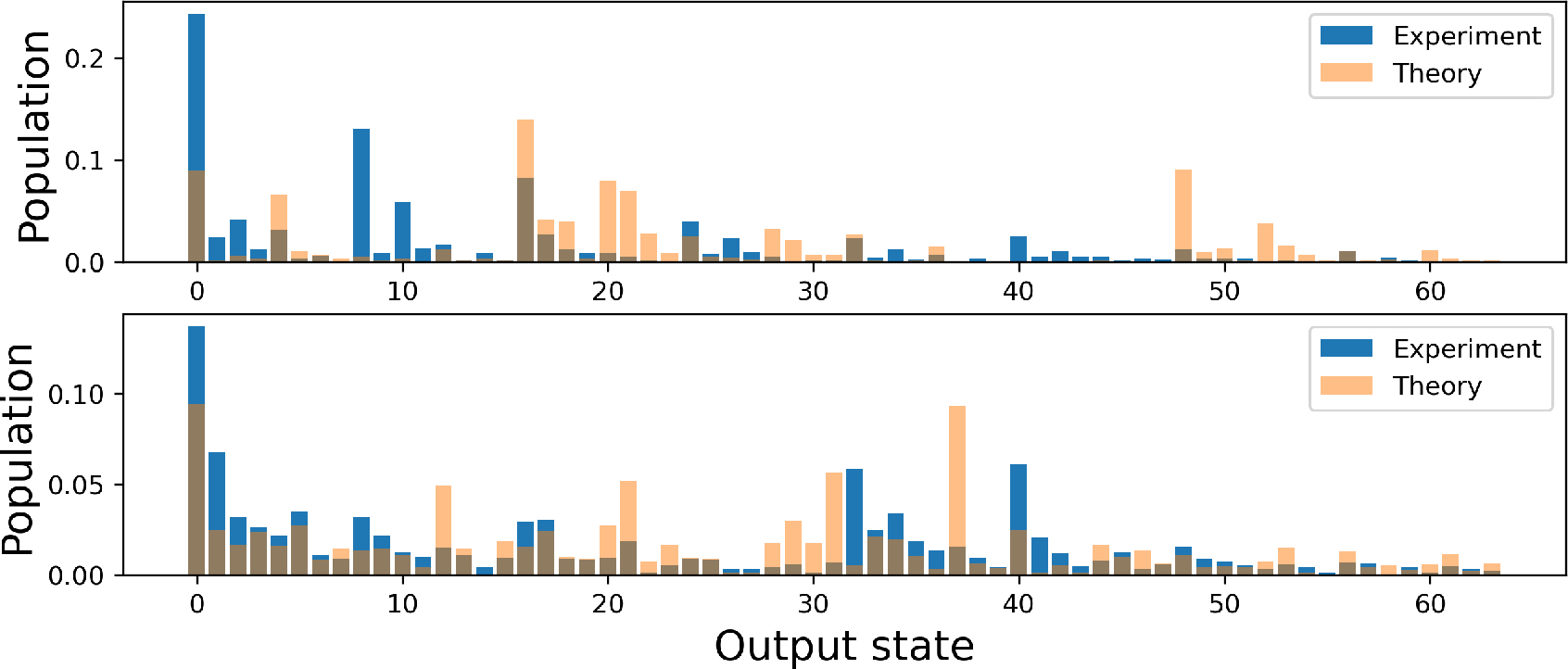
Figure 7.
Output states probabilities for circuits 1 and 6 from Table 5 sampled by the quantum processor and the noiseless emulator. Output states are numbered as a decimal representation of the output bitstrings. The first qubit corresponds to the high-order digit in the bitstrings. Each histogram is an average of 2000 shots.
In Figure 8 we also show analogous output probability distributions for the circuits where we use only 5 qubits to factorize number 437. It can be seen that the sampling fidelity is generally higher than for a 6 qubit case due to smaller circuit depth. However, for such a small problem size no quantum advantage over random sampling was observed.
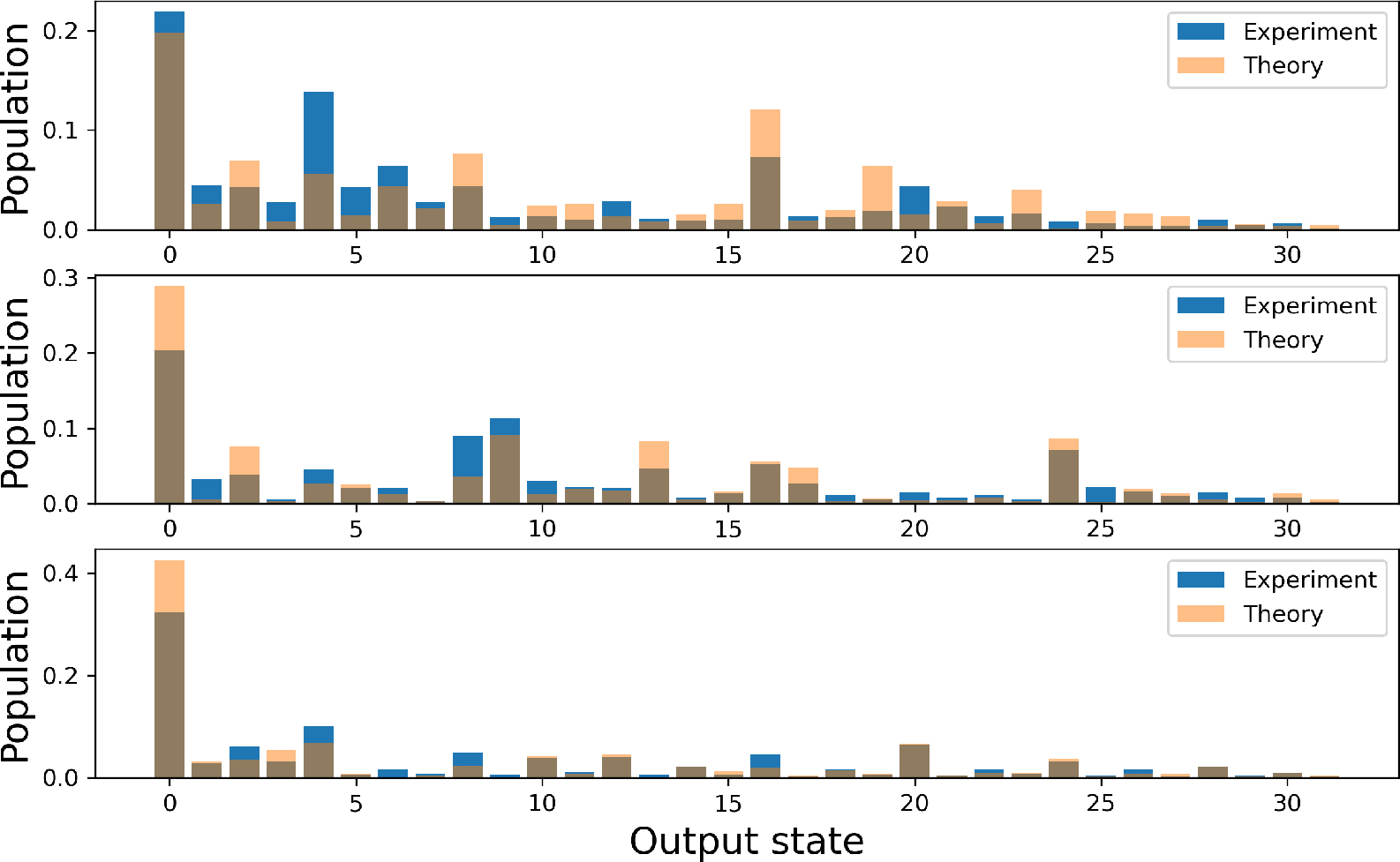
Figure 8.
Output states probabilities sampled by the quantum processor and the noiseless emulator for a set of circuits used to factorize number 437 using 5 qubits. Output states are numbered as a decimal representation of the output bitstrings. The first qubit corresponds to the high-order digit in the bitstrings. Each histogram is an average of 2000 shots.
Factoring Algorithm Details
Here we provide the description of the factoring algorithm adapted from [29]. The formal detailed description of Babai’s algorithm for CVP-approximation subroutine is presented in Algorithm 1. Overall factoring procedure is presented in Algorithm 2. Further, we consider the QUBO refinement of CVP-approximation. Generally, for any CVP defined by a lattice B = {bij} and a target vector tj, we need to find integer coefficients ai ∈ ℤ minimizing . Babai’s algorithm (however, it can be replaced by any other real approximation algorithm) provides a real-valued approximation ci ∈ ℝ. Then the rounded values ⌈ci⌋ are being taken as an approximate integer solution. Let us define variables that specify the rounding side:
Then the problem of choosing the side of each rounding has the form:
which is a QUBO problem with integer coefficients and can be approximately solved by the fpQAOA algorithm.Algorithm 1 Babai’s CVP algorithm Babaiδ (adapted from [29])
Require: b1,…, bn ∈ ℤn+1 ▷ Basis vectors of the considered lattice Λ
1: t ∈ ℤn+1 ▷ Target vector
2: δ ∈ (0.25,1) [δ = 3/4 by default] ▷ Parameter of the LLL-reduction
Ensure: c = (c1,…, cn) ∈ ℤn ▷ Rounded coefficient of the solution in LLL-reduced basis
3: ¯ = (μ1,…, μn) ∈ ℝn ▷ Unrounded coefficient of the solution in LLL-reduced basis
4: (d1,…,dn) ▷ LLL-reduced basis
5: d1 dn ← LLLδ(b1,…,bn) ▷ Constructing LLL-reduced basis via standard procedure
6: ← Gram-Schmidt orthogonalization of (d1,…, dn)
7: b ← t
8: for j = n, n – 1,…, 1 do
9:
10: cj ← ⌈μj⌋
11: b ← b – cj dj
12: end for
13: return c, μ, (d1,…, dn)
Algorithm 2 fpQAOA-enhanced factorization algorithm (adapted from [29])
Require: N ∈ ℕ+ ▷ RSA integer to be factorized
1: n ∈ ℕ+ ▷ Number of qubits used in the QAOA
2: B2 ∈ ℕ+ (s.t. B2 ≥ n, pB2 < N ▷ Size of a factor base used for checking sr-pairs
3: c ∈ ℝ+ ▷ Rounding parameter
4: δ ∈ (0.25,1) [δ = 3/4 by default] ▷ Parameter of the LLL-reduction in Babai’s algorithm
5: sort ∈ {True, False} [sort = False by default] ▷ Rearranging parameter for Babai’s algorithm
Ensure: p, q ∈ ℕ or Fail ▷ Factors of N
6: i ← 0 ▷ Initialize a counter for found relations
7: while i < n + 1 do ▷ Accumulating sr-pairs
8: Fix a random permutation f : [1,…, n] ↦ [f(1),…, f (n)]
9: for j = 1,2,…, n do ▷ Setting lattice’s basis vectors
10:
11: bj [n + 1] ← 10c ln pk
12: end for
13: t[k] ← 0 for k = 1,2,…, n, t[n + 1] ← 10c ln N ▷ Setting the target vector
14: c, μ, (d1,…, dn) ← Babaiδ(b1,…, bn; t) ▷ Applying Babai’s algorithm to obtain rounded (c) and unrounded (μ) coefficients of solution in the LLL-reduced basis d1,…, dn
15: x ← fpQAOA(c; μ; d1,…,dn; t) ▷ Applying the QAOA to obtain corrections xi ∈ {± 1,0 }
16: ▷ Updating CVP solution
17: ▷ Rewriting the updated CVP solution in the initial basis
18: , Constructing candidates for an sr-pair
19: if u – v · N is PB2-smooth and then ▷ A new sr-pair has been found
20: ui ← u, vi ← v ▷ Adding the sr-pair
21: ▷ Decomposing ui and ui – Nvi in PB2
22: i ← i + 1 ▷ Increasing counter and proceed to the next permutation
23: end if
24: end while
25: mod 2 ▷ Constructing the system of linear equations
26: Ker[(ai,j)] = Span(τ1,…, τm) ▷ Extracting linearly independent solutions
27: for τ = τ1,…, τm do ▷ Looking through the solutions
28: (mod N) ▷ Constructing Xτ satisfying
29: if Xτ ≢ ± 1 (mod N) then ▷ Success!
30: return gcd(Xτ + 1, N),gcd(Xτ – 1, N)
31: end if
32: end for
33: return Fail▷ No solutions found