
The integration of renewable energy sources (RESs) in modern power systems provides a practical solution to challenges associated with energy scarcity and environmental degradation. Since wind energy and solar energy are naturally complementary, effectively combining these two sources will enhance the reliability and efficiency of the power supply while significantly reducing carbon emissions. However, the inherent intermittency of these sources introduces substantial challenges to grid stability (Luukkanen et al., 2023), frequency regulation challenges in isolated grids (Matos et al., 2025), disturbance in power quality (Lata-García et al., 2024) and inefficient capacity utilisation (Bhutto, 2024).
Traditional solutions, such as lithium-ion batteries, which have response times >100 ms (Emon et al., 2023) and gas peaker plants, provide limited efficacy in addressing these challenges due to either their slow responsiveness or their associated emissions. This gap has catalysed research into hybrid systems that incorporate inertial storage technologies. Flywheel energy storage systems (FESS) have emerged as a promising solution, offering response times <20 ms and more than 100,000 cycles of durability (Fernandez et al., 2024). These characteristics make FESS particularly effective in alleviating the impacts of high-frequency renewable intermittency while simultaneously enhancing grid synchronisation (Younsi et al., 2023).
Recent advancements in hybrid wind-photovoltaic (PV) systems with integrated energy storage have led to three key architectural paradigms for addressing the intermittency of RESs (Morales-García et al., 2023). The first and most prevalent approach is the centralised DC-bus system, which has demonstrated operational efficiencies between 93% and 96% due to its common DC interconnection in large-scale grid applications (Anvari-Moghaddam et al., 2025). Enhancements, such as the torque-optimised MPPT design by Baala and Bri (2020), have been shown to improve wind energy capture by 8–12 percentage points compared with traditional systems. However, this architecture is inherently limited by vulnerabilities associated with single-point failures, particularly in fault conditions that persist for >500 ms (Li et al., 2021). By contrast, decentralised AC-coupled systems offer considerable modularity through plug-and-play functionality, facilitating flexible capacity scaling, a crucial advantage for distributed generation frameworks (Shafiullah et al., 2022). According to IEEE 1547.2-2023, compliance testing reveals that these systems often exhibit total harmonic distortion (THD) levels exceeding the 2.5% threshold, underscoring the need for improved filtering solutions. This requirement typically raises capital costs by 15%–20% (I.S.C. Committee, 2016). At the forefront of technology, hybrid DC/AC layered systems integrate both approaches by leveraging DC sub-grids alongside AC-coupled FESS (Hamrouni et al., 2019).
On the contrary, recent developments in intelligent control systems have become crucial for tackling the operational issues of renewable-based microgrids that utilise FESS (Kechida et al., 2024). Contemporary control architectures often feature a hierarchical framework that includes primary droop control for regulating voltage and frequency over sub-second intervals, model predictive control (MPC) for optimising setpoints across 15–30 s periods, and energy management systems (EMSs) that coordinate storage activity with load predictions (Serat et al., 2024). Analyses indicate considerable differences in performance across various control methods: traditional proportional-integral-derivative (PID) controllers show response times ranging from 120 ms to 300 ms with a THD of 3.2%, whereas fuzzy logic systems can achieve quicker responses of 50–80 ms with a reduced THD of 2.1% (Öhrström et al., 2025). Adaptive MPC has been shown to outperform with response times of just 20–40 ms and a THD of only 1.5%. Nonetheless, three significant challenges remain in current research: first, instability during mode shifts in 0.5–2 s grid-islanding scenarios, second, conflicting demands between quick frequency response and prolonged energy arbitrage, and third, the threat of cybersecurity issues that can lead to latency spikes of up to 230 ms in compromised systems (Roumeliotis et al., 2024). New solutions appear promising, with hybrid fuzzy-MPC controllers obtaining a tracking accuracy of 98.2%, digital twin technologies cutting computational latency by 40%, and blockchain-based communication offering verification times <5 ms (Dunna et al., 2024). These innovations underscore the necessity for advanced control frameworks that can effectively manage the multi-timescale dynamics of hybrid PV-wind-flywheel systems while ensuring grid stability and cybersecurity, an area that our proposed multi-agent control system aims to address specifically.
Research on hybrid renewable energy systems (RES) has been a prominent topic in various published studies. However, many of these evaluations primarily revolve around the operational conditions of hybrid RES featuring simpler topologies. The investigations were limited to a narrow range of operational modes and utilised basic control algorithms. Xu et al. (2023) outline the classifications and architectures of hybrid RES, while the optimisation methods for the sizing of their components are discussed in Ullah et al. (2024). An analysis of systems incorporating wind, PV, supercapacitors and batteries can be found in Chakir and Tabaa (2024). Anvari-Moghaddam et al. (2025) explored hybrid RES in standalone configurations with DC loads, while other studies (Fernandez et al., 2024) focused on systems equipped with AC loads. Several articles are dedicated exclusively to the operation of hybrid RES in standalone mode neglecting the topic of energy management strategies (Al-Rawashdeh et al., 2023). Most of the research has concentrated on systems utilising a simple topology with a machine-side converter linked to a permanent magnet synchronous generator (PMSG) (Gajewski and Pieńkowski, 2016).
This research introduces an advanced intelligent control system and optimisation framework for managing energy in an on-grid hybrid renewable generation (OG-HRG), including a FESS. This paper is organised as follows: Section 2 describes the integrated architecture and provides detailed mathematical models for the PV array, wind turbine (WT) dynamics and flywheel operation. Section 3 proposes a new control framework utilising a maximum power point tracker (MPPT) based on fuzzy logic Control (FLC) algorithms and sliding mode control (SMC), along with a comprehensive seven-mode energy management strategy. In Section 4, simulation results from key operational scenarios are presented, showing the stability of the DC bus within a deviation of ±0.005 V and an impressive renewable resource utilisation efficiency of 92.3%. Finally, Section 5 discusses implications for grid integration and potential future research avenues, including hardware-in-the-loop validation opportunities.
The schematic diagram presented in Figure 1 depicts the architecture of the proposed OG-HRG. This system integrates a photovoltaic generator (PVG) paired with a DC–DC boost converter, a WT with a PMSG in conjunction with a machine-side AC–DC converter and a FESS integrated with an AC–DC conversion system. The primary reason for utilising a flywheel in dynamics is its exceptionally high-power density and nearly instantaneous response time, making it perfect for handling rapid fluctuations in power demand and supply.
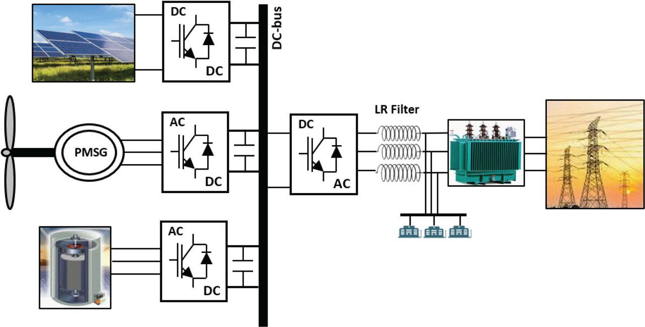
The architecture of the proposed OG-HRG. OG-HRG, on-grid hybrid renewable generation.
The flywheel is ideal for high-power, rapid-cycling applications, with a lifespan exceeding 20 years and more than 100,000 charge–discharge cycles. By contrast, typical lithium-ion batteries only last about 5,000 cycles. Flywheels respond in <100 ms, providing quick grid stabilisation, and both technologies have similar round-trip efficiencies of around 90%. However, the flywheel’s durability and fast power delivery make it the best choice for frequency regulation and demanding applications requiring long-term reliability.
All the components of the structure in Figure 1 are modelled by Eqs (1)–(13) and then integrated in a dynamic Simulink model (MATLAB environment).
The mathematical model of a PVG with Np parallel panels and Ns series cells is shown in Eq. (1) (Xu et al., 2023) as follows:
The PV current and voltage The diode current The PV array series and parallel resistors The panel ideality factor The electron charge The Boltzmann constant The PV array temperature
The WT transforms the kinetic energy of the wind into the mechanical rotational energy of its blades. The mechanical power, Pt, generated by the WT is represented by Eq. (2) (Aloo et al., 2023) as follows:
The space covered by the rotor blades (R is the diameter of the turbine blades) The density of air The ratio of the tip speed The angle of the blade pitch The WT’s power coefficient The velocity of the wind
The tip speed ratio of the WT is expressed as shown in Eq. (3):
The turbine power coefficient Cp relies on a complex relationship involving two variables: the tip speed ratio and the blade pitch angle. The power coefficient Cp can be approximated using Eqs (4) and (5) as follows:
The mathematical model of PMSG is based on several fundamental assumptions: the three-phase stator windings are symmetrical and distributed sinusoidally throughout the air gap of the machine, the effects of magnetic hysteresis and saturation are not considered and no damping windings are included. In the constructed model, the variables are expressed in the synchronous rotating dq-reference frame, with the d-axis aligned to the direction of the flux vector of the permanent magnet rotor. The mathematical equations governing the PMSG are formulated within the conventional dq-reference frame, which rotates in synchronisation with the electrical angular velocity of the rotor. The mathematical model of this system is given in Eq. (6) (Yadav and Balasubramaniyan, 2025) as follows:
The dq elements of the stator voltage vector The dq elements of the stator current vector The dq elements of the stator flux vector The magnetic field created by the permanent magnets The rotor’s electrical and mechanical angular velocity of the PMSG The resistance of the stator phase The stator inductances for both direct and quadrature components The quantity of pole pairs in a PMSG
The electromagnetic torque of the PMSG is expressed in Eq. (7) as follows:
The expression for the mechanical motion ωm of the WT system is represented in Eq. (8) as:
A FESS combines a flywheel, a PMSG and an AC–DC converter. This system operates in charging and discharging modes:
In charging mode, energy is transferred from the DC bus to the flywheel: in this first mode, the PMSG operates as a motor.
In discharging mode, energy is transferred from the flywheel to the DC bus: in this second mode, the machine operates as a generator.
However, the direction of the current changes depending on the machine’s operating mode.
The stored energy Ev in the flywheel is expressed in Eq. (9) (Elkholy et al., 2024) as follows:
On the other hand, materials with high tensile strength σmax are required to counteract centrifugal forces and enable operation at elevated peripheral speeds. The significant energy content is expressed in Eq. (10) as follows:
With ρ as the material’s density, M as the total flywheel mass and K being a constant determined by the flywheel’s particular shape.
Typically, the PV system’s output voltage Vpv is insufficient to meet the DC bus voltage requirement Vdc. To bridge this gap, a boost DC–DC converter steps up Vpv to the required Vdc level. The converter’s dynamic behaviour is modelled in Eq. (11) (Chakir and Tabaa, 2024) as follows:
The grid integration of RESs is achieved through a three-phase inverter that performs DC–AC conversion. The inverter’s output voltages (Vs1, Vs2, Vs3), as described by Eq. (12), are directly controlled by the switching signals (k1, k2, k3) that modulate the power devices (Younsi et al., 2022) as follows:
To ensure proper grid current injection, an L-type filter (Rf, Lf) interfaces the inverter with the utility grid. The dq axis dynamic model of this filter, derived with (Id, Iq) as states and (Ed, Eq) as inputs, is formulated in Eq. (13) as follows:
Rf and Lf characterise the grid filter’s resistive and inductive components. The grid operates at angular frequency ω, with Kd and Kq serving as the decoupled control inputs for the inverter’s dq coordinate frame.
The proposed OG-HRG utilises a control strategy that incorporates fuzzy logic control (FLC) for maximum power point tracking (MPPT) to optimise the extraction of PV energy, along with rotor field oriented control (RFOC) to maximise wind energy capture and manage the FESS. To manage the power flow, SMC is employed at the inverter grid interface. Figure 2 illustrates the control strategy of the OG-HRG.
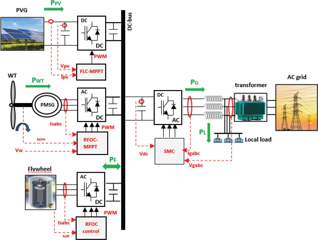
The control strategy of the OG-HRG. OG-HRG, on-grid hybrid renewable generation; PMSG, permanent magnet synchronous generator; PVG, photovoltaic generator; RFOC, rotor field oriented control; SMC, sliding mode control.
The main purpose of employing both fuzzy logic control and a sliding mode controller together is to establish a robust hierarchical control system. This system optimises energy extraction from the PV array while ensuring that the collected energy is supplied to the grid efficiently, effectively and reliably.
FLC excels in microgrids and real-time systems, offering fast response (<0.5 s) and reliable partial shading performance, though requiring rule tuning. Artificial neural networks (ANN) achieve >99% accuracy in large solar farms but need extensive training data, limiting adaptability (Kaur et al., 2023). Particle swarm optimisation (PSO) suits off-grid systems where its slower convergence (2–5 s) is acceptable, though it struggles with rapid shading changes. FLC balances cost and performance for embedded systems, ANN dominates data-rich environments, while PSO remains a niche for offline optimisation. The choice depends on system needs: speed (FLC), precision (ANN) or flexibility (PSO).
For converting the electrical energy generated by the PV array, a DC–DC boost converter topology is utilised. The schematic for this type of converter is shown in Figure 3.
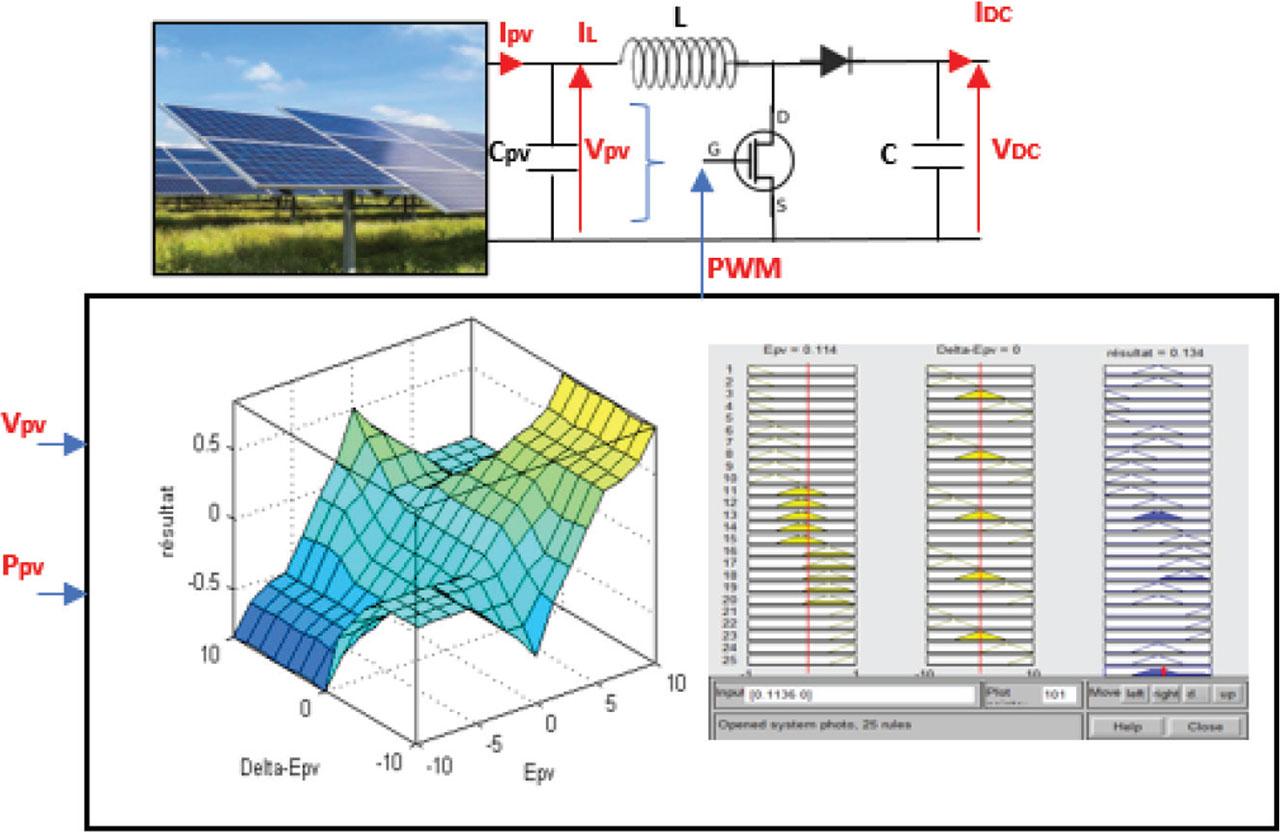
The configuration of the FLC-based MPPT.
The FLC-MPPT algorithm optimises PV power extraction by dynamically adjusting the DC–DC converter’s duty cycle. It works by sampling PV voltage (V) and current (I) to calculate power (P), computing power (ΔP) and voltage (ΔV) gradients, fuzzifying inputs into linguistic terms (Negative/Zero/Positive), processing through a fuzzy rule base to determine duty cycle adjustments, defuzzifying the output to update the PWM signal and repeating until maximum power point (MPP) is achieved (Pande et al., 2021).
The structure of the FLC strategy is described in Figure 4.
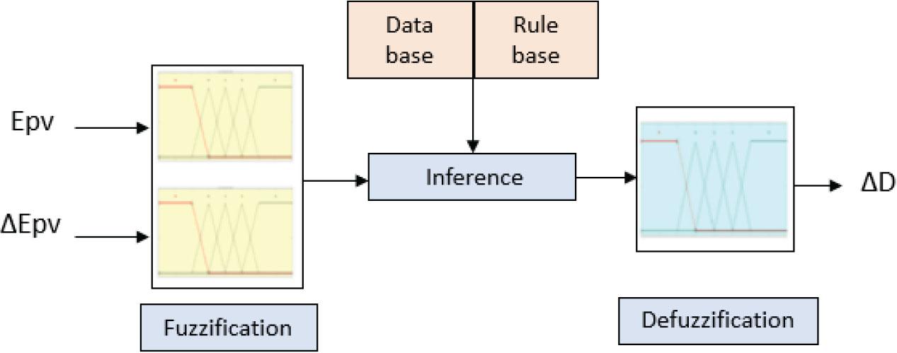
Structure of the FLC-based MPPT controller.
In this study, the inputs of the fuzzy logic controller (FLC) are the slope of the (Ppv–Vpv) characteristic of the PVG, denoted as Epv(k), and the slope variation ∆Epv(k) between two time instants k and k−1, which is expressed in Eq. (14) as follows:
The fuzzy controller generates outputs ΔD, which are then converted into numerical values, and the duty cycle D(k) is determined using Eq. (15) as follows:
MPPT control determines the turbine’s optimal speed by evaluating its power coefficient characteristic CP(λ, β), ensuring operation at peak efficiency, establishing the power–speed characteristic curve that correlates the maximum extractable wind power (Pt−m) with its corresponding optimal rotor speed (Ωt−m). CP designates the power coefficient of the WT, λ refers to the ratio of the tip speed and the blade pitch angle is denoted by β.
The MPPT detects the points where power is at its highest for different wind speeds. The summit of the CP (λ, β) curve signifies the greatest amount of power that can be extracted from the wind generator. For low-power uses involving WTs with fixed pitch, the MPPT power regulation is solely handled by the converter control, which modifies the alternator’s output parameters, such as current and voltage, influencing the speed of the rotor. The power coefficient is maximised at this particular β value and a particle speed of λ (λm), which is stated in Eq. (16) (Rekioua et al., 2024) as follows:
The maximum value of the CP (β = 0) is given in Eq. (17) as follows:
In this case, the expression for the maximum of the turbine’s power is expected as given in Eq. (18):
The expression for the maximum rotation speed of the aerodynamics within the wind speed range from the starting speed to the nominal speed is given in Eq. (19) as follows:
The corresponding maximum aerodynamic torque is given in Eq. (20) as follows:
The control scheme for the FESS is shown in Figure 5.
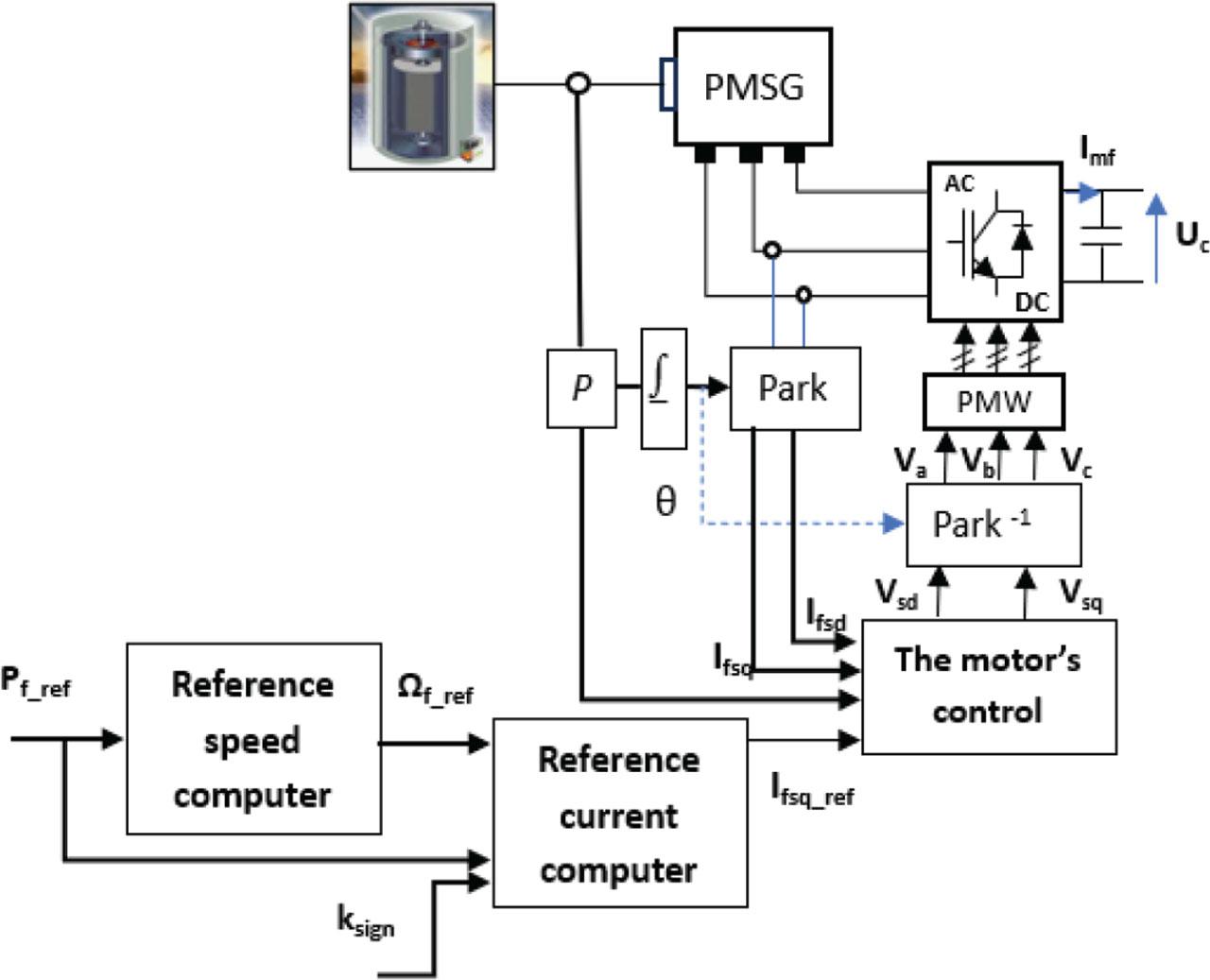
The control scheme for the inertia-driven energy storage unit. PMSG, permanent magnet synchronous generator.
The reference stator current component on the q-axis is expressed in Eq. (21) (Younsi et al., 2023) as follows:
When the storage system is charging, power is transferred from the DC bus to the flywheel (ksign = −1). In contrast, when the storage system discharges, power is transferred from the flywheel to the DC bus (ksign = 1). The standby mode corresponds to ksign = 0. These three operating modes are shown in Figure 6.
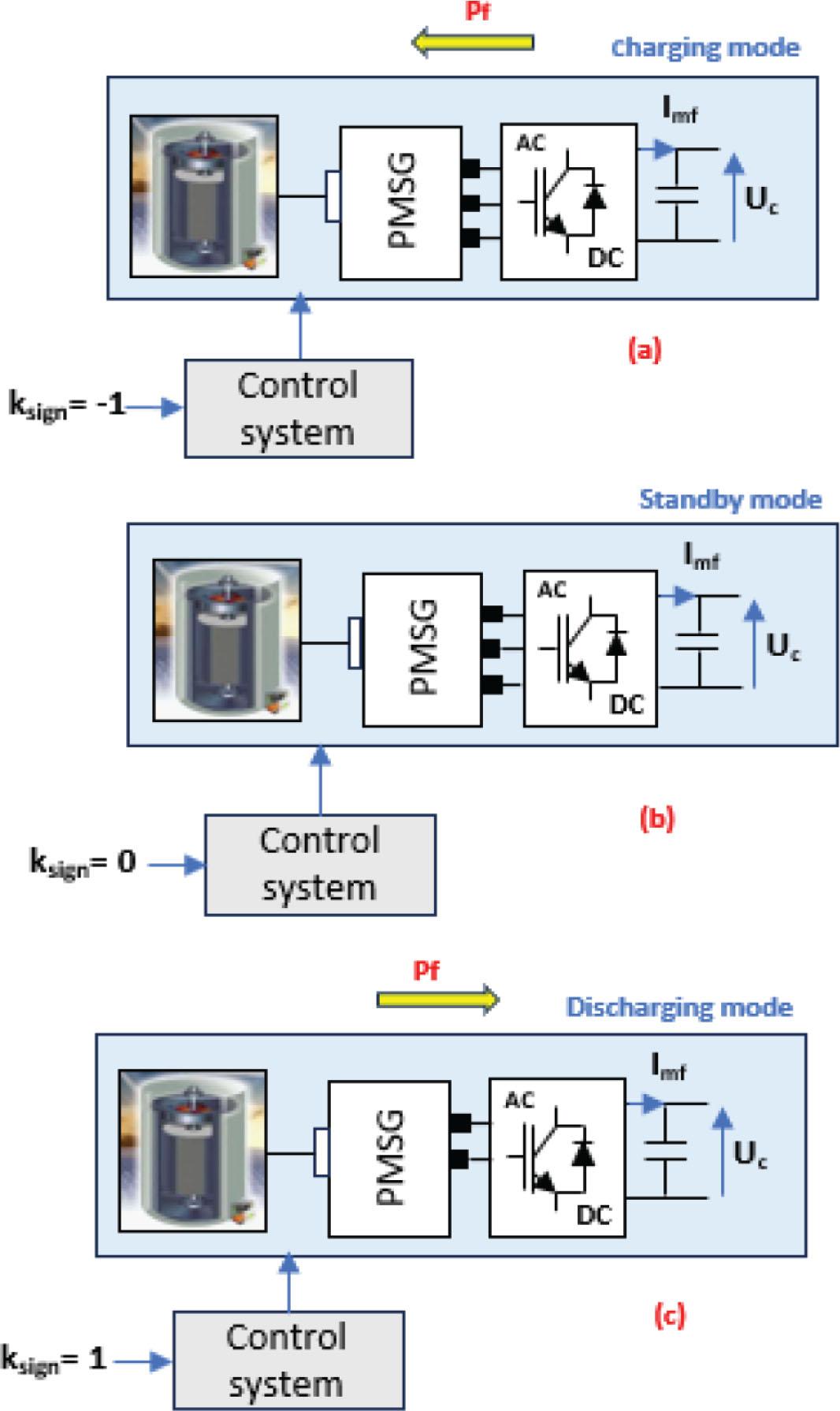
The FESS operating modes. FESS, flywheel energy storage system; PMSG, permanent magnet synchronous generator.
The reference speed of the flywheel is determined in Eq. (22) as follows:
Through SMC, the inverter achieves two primary objectives (Šmídl et al., 2023):
Maintaining current waveforms with low THD;
Ensuring precise phase alignment with the grid voltage.
The standard sliding mode controller configuration for this application is depicted in Figure 7.
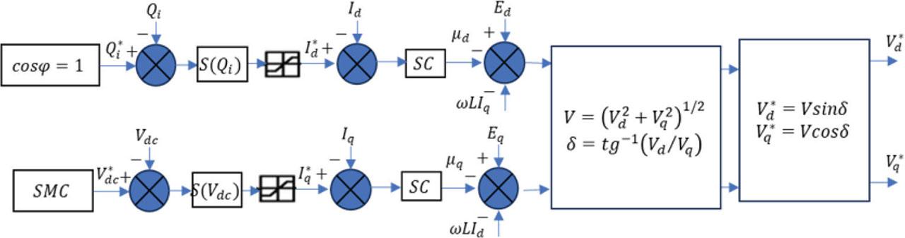
The architecture of the SMC controller. SMC, sliding mode control.
The EMS aims to continuously match the supply from renewable sources with demand from loads and charging/discharging of storage units. The OG-HRG can operate in several scenarios depending on climatic conditions, stored energy, local load demand and network status. This operation improves the system performance in terms of quality of service and security.
The design of the EMS is given in Figure 8.
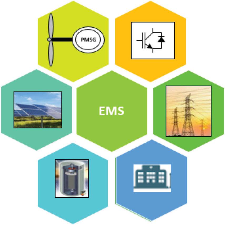
The EMS of the OG-HRG. EMS, energy management system; OG-HRG, on-grid hybrid renewable generation.
Table 1 illustrates the different operating modes (Mi) and sub-modes (Mij) of the OG-HRG. Mode M5 produces two sub-modes, which are determined by the direction of power flow from the grid. PREN, PL, PF and PG denote the power generated by the PVG and the WT, the power used by the load, the power exchanged with the flywheel and the power received from or delivered to the grid, respectively. If any system component is disconnected, its power output becomes zero. The energy balance of the system is assessed based on the actions of the two active components of the set-up (RESs and the grid), the storage system and the load status. The availability of a hybrid system component is represented by a logical state (1), while unavailability is indicated by a logical state (0).
The power flow operating modes.
| No. | Operating mode | Keys state | Energy movement | Power balance | ||||||
|---|---|---|---|---|---|---|---|---|---|---|
| K1 | K2 | K3 | EREN | EG | EL | EF | Composition | System state | ||
| 1 | M1 | 0 | 0 | 0 | 0 | 0 | 0 | 0 | Maintenance | – – – – – – – – – – |
| 2 | M2 | 0 | 1 | 1 | 0 | <0 | >0 | 0 | Grid-load | PG = PL |
| 3 | M3.1 | 0 | 1 | 0 | <0 | - | >0 | >0 | PV + WT—Fl—L (disconnected mode) | Storage: PREN = PL + PF |
| 4 | M3.2 | 1 | 0 | 1 | <0 | - | >0 | <0 | PV + WT—Fl—L | Discharge: PREN = PL − PF |
| 5 | M4 | 1 | 1 | 0 | <0 | 0 | 0 | 0 | PV + WT—grid | Direct injection to grid PREN = PG |
| 6 | M5.1 | 1 | 1 | 1 | <0 | >0 | >0 | 0 | PV + WT—grid-load | PREN > PL |
| PREN = PG + PL | ||||||||||
| 7 | M5.2 | 1 | 1 | 1 | <0 | <0 | 0 | 0 | PV + WT—grid-load | PREN < PL |
| PREN = PL − PG | ||||||||||
PV, photovoltaic; WT, wind turbine.
Seven scenarios exist based on the state of the power flow, as described in Table 1.
According to Table 1, we identify the following scenarios for energy supply:
In two operational modes (M3.1, M4) and one sub-operational mode (M5.1), RESs (wind/PV) function as generators while the other components serve as receivers.
IIn operational mode M3.2, the flywheel operates as a generator.
IIn operational mode M2, the grid functions as a generator with the RESs disconnected.
IIn only one sub-operating mode M5.2, energy is simultaneously provided by both sources (renewable energy and the grid).
IIn operational mode M1, all components of the system are disconnected.
The suggested OG-HRG power management algorithm relies on the subsequent strategy:
If PL < PREN and the grid is active then:
- -
The local demand is supplied;
- -
The grid gets the excess energy.
- -
If PL < PREN and the grid is inactive (disconnected due to a fault) then:
- -
The local load is supplied;
- -
Power is delivered from the DC bus to the flywheel: charging mode.
- -
If PL = PREN and the grid is active or inactive (islanded mode) then:
- -
The local load is supplied;
- -
The grid is not part of the power transfer process;
- -
No power is exchanged between the bus and the flywheel: standby mode.
- -
If PL > PREN and the grid is active then:
- -
The local load is supplied;
- -
The grid provides the power deficit;
- -
No power is exchanged between the bus and the flywheel: standby mode.
- -
If PL > PREN and the grid is inactive (disconnected due to a fault) then:
- -
The local load is supplied;
- -
The grid is not involved in power transfer;
- -
Power is delivered from the flywheel to the DC bus: discharging mode.
- -
The flowchart of the EMS is described in Figure 9:
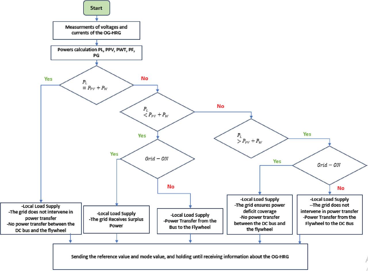
The flowchart of the EMS of the OG-HRG. EMS, energy management system; OG-HRG, on-grid hybrid renewable generation.
In this section, we provide a detailed analysis of a set of graphs that illustrate the various operating scenarios of the overall system. These scenarios are effectively managed through appropriate commands and are continuously monitored by the energy manager. The selected wind profile is illustrated in Figure 10, while the solar intensity is maintained at 600 W/m2. During this timeframe, the RES supplies approximately 2,650 W of power.
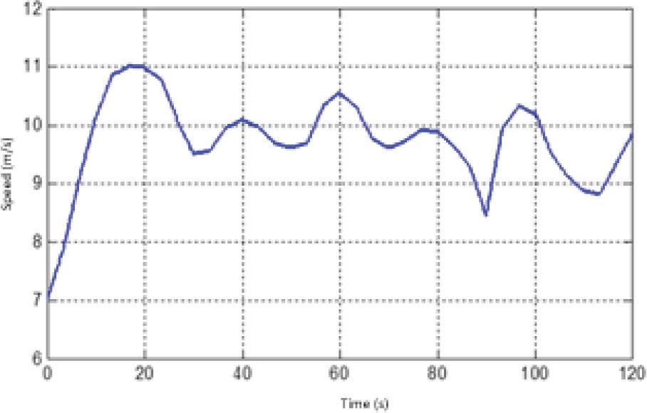
The wind profile.
Additionally, the load profile exhibits variability, as outlined in Table 2. This comprehensive approach enables us to better understand the dynamics of the system and optimise its performance.
The power balance for each operating mode.
| Operating mode | M3.1 | M3.2 | M3.1 | M5.1 | M5.2 | M4 | M5.1 |
|---|---|---|---|---|---|---|---|
| Time (s) | 13.5–14 | 14–14.5 | 14.5–15 | 15–15.5 | 15.5–16 | 16–16.5 | 16.5–17 |
| PL(W) | 960 | 2,750 | 960 | 960 | 3,960 | 0 | 960 |
Figure 11 illustrates the supplied and absorbed powers of subsystems for the different operating modes. From t = 13.5 s to 15 s, the hybrid system operates in autonomous mode. The network is inactive, and the power supplied by the flywheel is assumed to be sufficient to compensate (absorb) the energy deficit (surplus) during this operating mode, which corresponds to M3.
Between 13.5 s and 14 s, the power supplied by the RES is approximately 2,650 W, while the load demand is equal to 960 W. The excess power of 1,690 W is sent to the flywheel. The flywheel operates in charging mode (M3.1).
Between 14 s and 14.5 s, the load demand is around 2,750 W. In this case, the flywheel operates in discharging mode to compensate for the estimated production-consumption power deficit of 100 W.
Between 14.5 s and 15 s, the load demand drops again to its initial state. The flywheel switches to its charging state to absorb excess power resulting from production and consumption.
From t = 15 s to 17 s, the hybrid system operates in connected mode. The manager activates the power control of the inverter and the MPPT command on the chopper. The flywheel becomes inactive and does not participate in energy exchange.
Between 15 s and 15.5 s, the power supplied by the OG-HRG is approximately 2,650 W while the load demand is equal to 960 W. The excess power of 1,690 W is sent to the grid. The system switches to M5.1 mode.
Between 15.5 s and 16 s, the load demand increases to reach 4,000 W. In this case, and in the absence of the flywheel, the grid compensates for the production–consumption power deficit. The system switches to M5.2 mode.
Between 16 s and 16.5 s, the load is disconnected, and all of the power generated by the OG-HRG is injected into the electrical grid. The system operates in M4 mode.
Between 16.5 s and 17 s, the load power becomes 960 W. The power supplied by the OG-HRG is greater than that of the load. However, excess energy is sent to the grid. The system returns to M5.1 mode.
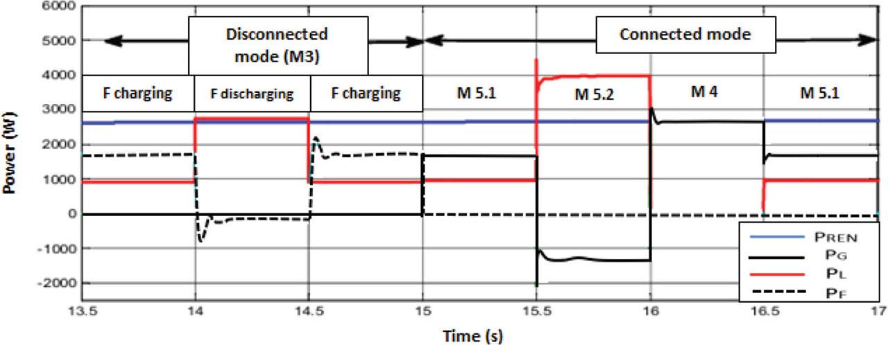
The powers supplied/absorbed by the subsystems for the different operating modes.
Figure 12 shows the variation of currents on the DC bus side, namely the current supplied by the OG-HRG corresponding to the maximum power, the direct current exchanged with the flywheel, as well as the current at the input of the inverter returned to the load and the grid. The current supplied by the OG-HRG is around 5 A. The current sent or withdrawn from the network depends on the load under the operating modes. In connected mode (M5.1, M5.2 and M4), the current sent to the alternating side presents disturbances each time the operating mode changes. This is due to the nature of the load, which is made up of a pump unit. Figure 13 shows the DC bus voltage, which varies around its reference imposed by the control. However, the simulated voltage deviates from its reference by ±0.005 V each time the operating mode changes. This is due to the start of the load and its temporary nature (asynchronous motor).
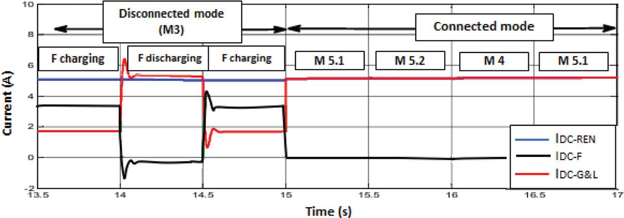
The variation of currents on the DC bus side.
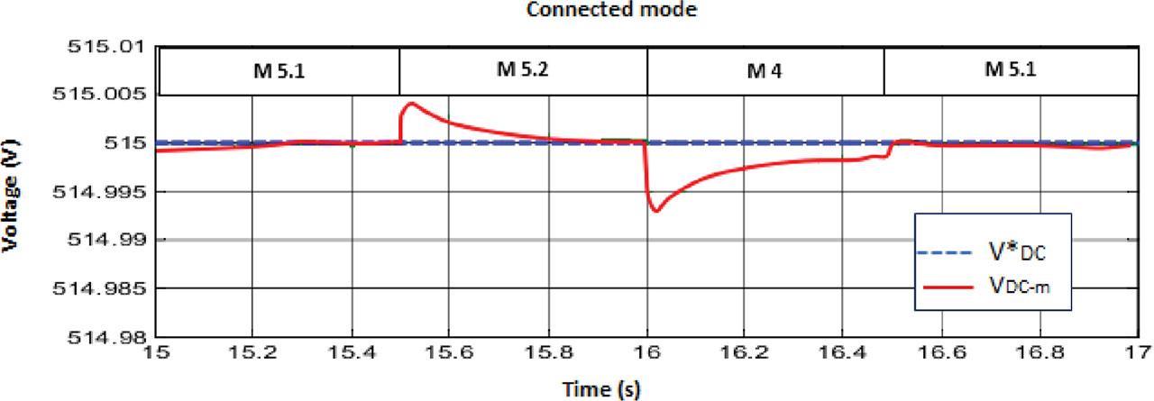
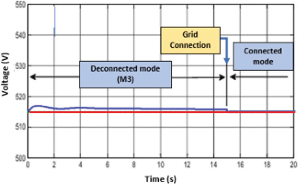
The variation of voltage on the DC bus side.
For a DC-bus voltage equal to 515 V, the maximum current supplied is around 3.95 A. This current is constant during the different operating modes. In island mode, part of this PV current is consumed by the load (1.75 A) and the balance (2.2 A) is stored in the flywheel to avoid increasing the bus voltage. Figure 14 shows that the bus voltage varies slightly around its reference.
The DC-bus voltage waveform.
In Figure 15, during the start-up phase, which lasts for 0.5 s, the amplitude of the current at the input of the inverter is of the order of 2.8 A. This current is consumed by the asynchronous motor during starting. Furthermore, the current injected into the flywheel is equal to 1.15 A. At t = 15 s, the inverter connects to the grid since the connection conditions are satisfied. However, the control system switches to power control mode. In this case, the DC bus voltage further converges towards its reference fixed at 515 V. The current returned to the flywheel is cancelled, and that at the input of the inverter goes from 1.7 A to 3.95 A. Part of this current is consumed by the load (1.75 A), and the other part is returned to the grid.
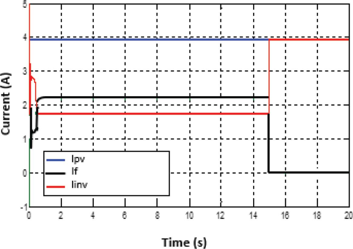
The PV, Flywheel and inverter current waveforms. PV, photovoltaic.
The profiles of active and reactive power injected into the grid are shown in Figure 16 ((a): active power PG and (b): reactive power QG).
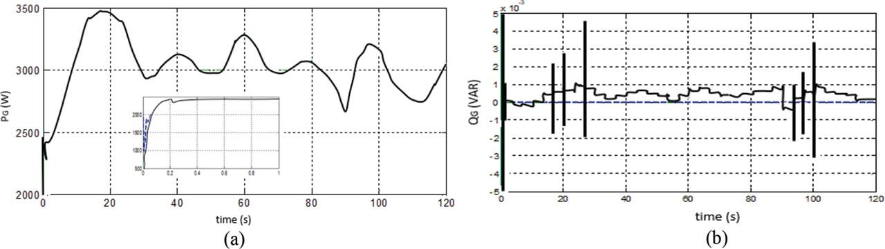
Profile of the active (a) and reactive (b) power injected into the grid.
Figure 17 shows the variation curves of the hybrid system’s power in grid-connected and islanded modes >20 s. During these different operational phases, the PV power remains at its maximum (2,040 W) since the MPPT control is not degraded.
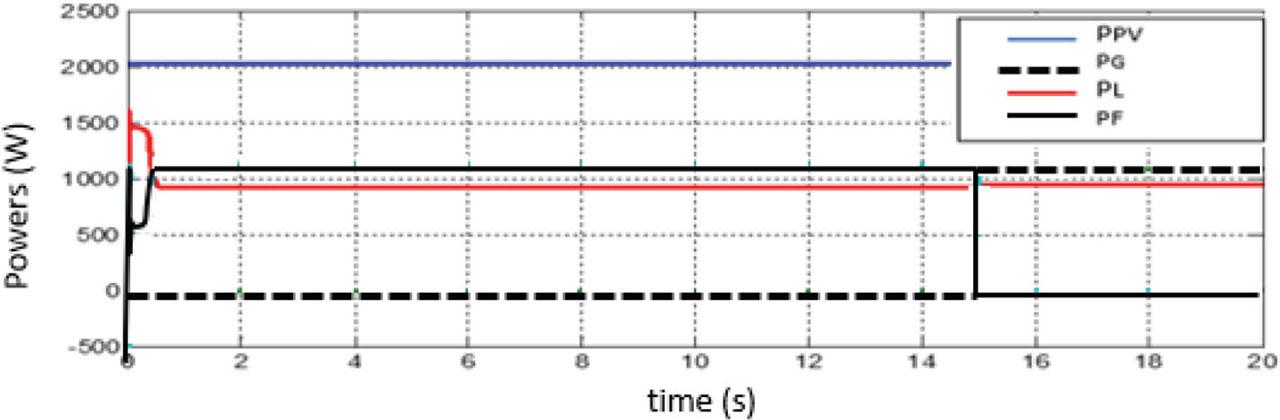
The power waveforms.
In the islanded mode, which lasts for 15 s, the power injected into the grid is zero, while the power consumed by the load at startup (an asynchronous motor with a rated power of 1 kW) is around 1.5 kW. The surplus power between generation and local consumption is sent to the flywheel (≈600 W). In steady-state operation, the power demanded by the machine is around 950 W, while the surplus (≈1,200 W) is stored in the flywheel.
At the moment of grid synchronisation, the power injected into the flywheel drops to zero, and the power injected into the grid increases from 0 W to 1,080 W. A slight discrepancy in the load power consumption is observed during synchronisation. This discrepancy arises from the transition to a power supply dictated by the grid voltage, which has a slightly higher amplitude than the voltage provided by the inverter in islanded mode.
Figure 18 shows the appearance of the direct and quadrature components of the currents and voltages (simulated and reference) Id (a), Iq (b), Vd (c) and Vq (d), controlling the inverter for the different operating modes.
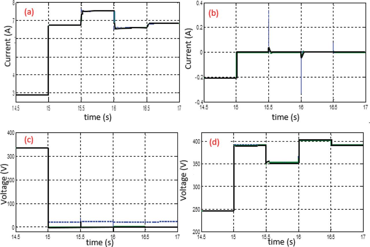
The direct and quadrature components of the currents and voltages Id (a), Iq (b), Vd (c) and Vq (d), (simulated and reference) waveforms.
The profiles of the output voltage and load current are displayed in Figure 19.
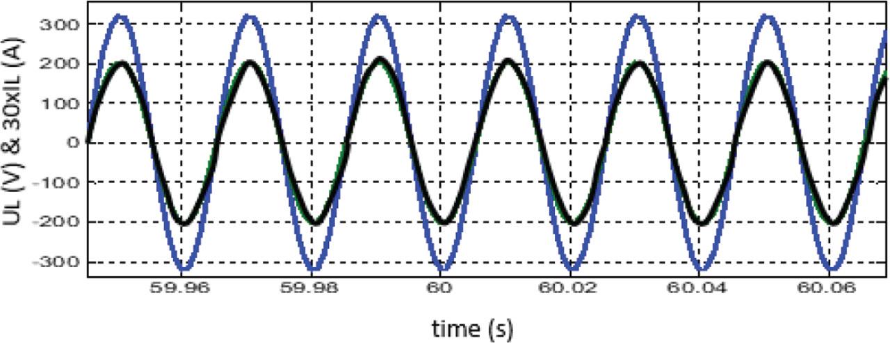
The load voltage and (30×) load current waveforms.
The developed control provides good dynamic performance with regard to voltage and current response. Likewise, it makes it possible to maintain the DC bus voltage constant, whatever the operating mode. In addition, the voltage and current injected by the inverter are always regulated, and the responses follow, without overshoot and static error, their references generated by the control system. The control system showed notable robustness (accuracy and speed) when varying the load and when switching from one mode to another. Table 3 provides a comparison of the proposed OG-REG with other studies.
Comparison with other studies.
| Paper reference | Energy source and storage | Performance summary |
|---|---|---|
| Our paper | Grid-connected PV/wind/flywheel | This system features a multi-layered control approach that combines FLC, PID control and SMC into a unified EMS. |
| Reference Lata-García et al. (2024) | Stand-alone PV/biomass/diesel/battery | The system consists of a 22 kW solar PV generator, a 1.5 kW biomass generator and a 12 kW diesel generator. Additionally, the battery bank includes 58 units, each with a capacity of 111 Ah, and the dispatch strategy employed is load tracking. |
| Reference Younsi et al. (2023) | Grid-connected wind/flywheel | This control system includes primary and secondary controllers. The primary stage uses a droop controller to optimise power flow in the resistive network, while the secondary stage employs an improved method to manage voltage and frequency fluctuations during signal disturbances. |
EMS, energy management system; PID, proportional-integral-derivative; PV, photovoltaic; SMC, sliding mode control.
This paper proposes an analysis and simulation study of an innovative OG-HRG system. The system under consideration includes a gearless WT with a PMSG, a PV array and a FESS. The research concentrated on the DC-coupled architecture of the multi-converter OG-HRG.
The system efficiently manages power flow to loads, adapting seamlessly to the varying operating conditions of RESs. The innovation of the proposed OG-HRG system lies in its integrated analysis, which is more comprehensive than the typical isolated assessments of individual components commonly found in the literature. This holistic approach enables a deeper understanding of the interactions within the system, leading to enhanced performance and stability.
In managing the operation of the PV system, an FLC MPPT algorithm has been applied to achieve the highest possible output of power generated by the PV system under varying conditions of solar irradiation and ambient temperature.
RFOC is applied for the PMSG, integrating the MPPT algorithm to achieve the maximum power generation from the WT. The RFOC is applied to the FESS to manage power flow during charging and discharging phases. The FESS was vital in alleviating power fluctuations and preserving grid stability.
The control of the grid-connected inverter is performed using an SMC approach, which guarantees stable regulation of the DC link voltage and efficient management of the power transfer between the RES and the electrical network. Thus, the incorporation of advanced control techniques guarantees optimal energy extraction and efficient functionality.
The proposed EMS successfully aligned energy production from renewable sources with load requirements and storage demands. The system’s performance was assessed under different operational scenarios, showcasing its ability to manage power flow and enhance grid stability.
MATLAB/Simulink simulations demonstrate significant improvements: 72% reduction in power fluctuations compared with battery-based hybrid systems, 85% decrease in CO2 emissions and operational stability across all seven operating modes (M1–M5.2). This unified approach simultaneously addresses both fast-timescale inertia requirements (via flywheel) and long-term energy balancing needs (through predictive EMS), thereby overcoming the major limitations of existing architectures.
This study highlights the significant potential for further enhancement and optimisation of hybrid renewable energy systems, with a particular focus on energy management strategies and the integration of additional storage technologies. Future research could delve into the scalability of the system for larger grids and the incorporation of diverse RESs. In conclusion, the proposed hybrid renewable energy system, featuring advanced control and energy management techniques, offers a robust solution for sustainable power generation. By blending wind, solar and flywheel storage technologies, this approach provides a reliable and efficient method to address the challenges associated with renewable energy variability, contributing to improved grid stability and more effective energy utilisation. Experimental validation will be addressed in future research.