
Future production of energy faces significant challenges. Furthermore, the energy requirements of emerging nations will increase to sustain their progress. The two primary types of power sources are non-renewable and renewable. Sources of renewable energy include geothermal, biomass, wind, sun and hydropower. Resources such as uranium, gas, oil and coal are examples of non-renewable energy sources (Ahmed and Salam, 2015; Anagreh et al., 2021). The use of non-renewable fossil fuels produces emissions of greenhouse gases, which worsen air pollution. Moreover, these fossil fuel resources are finite and will eventually be exhausted. As a result, many countries are committed to exploring renewable energy sources that are sustainable, cost-effective and environmentally friendly (Koofigar, 2016). By harnessing these innovative energy solutions, we can effectively eliminate the release of harmful greenhouse gases into the environment, pollute less or have any inherent risks than fossil fuels (Kumar, 2015; Liu et al., 2008). The use and advancement of photovoltaic (PV) energy are on the rise globally. One of the promising applications of this renewable energy source is PV pumping, which is particularly beneficial in rural areas with high levels of sunlight and no access to an electric grid (Dharmendra and Javed, 2023; Rim et al., 2020). Solar energy is derived from the electromagnetic energy captured by photosensitive cells from the sun’s radiation. This process converts electromagnetic radiation into electricity through the PV effect (Rezk et al., 2019). The efficiency of PV systems can be significantly improved using the maximum power point tracking (MPPT) techniques, which optimise performance based on the electrical characteristics and configuration of the PV cells (Hichem et al., 2019; Nihat, 2023).
Numerous research studies have explored and documented MPPT algorithms. Traditional techniques, such as the incremental conductance (INC) algorithm and the perturb and observe (P&O) algorithm (Hayat et al., 2022; Seba et al., 2023), have been extensively investigated and are among the most commonly employed methods.
Although conventional MPPT approaches are simple and effective under stable weather conditions, they often struggle to maintain accuracy near the maximum power point (MPP) and can be less suitable for large-scale solar power systems (Sahu et al., 2022; Yassine et al., 2022). These traditional methods tend to exhibit ripples close to the MPP, which limits their performance. As a result, researchers are working globally on developing more advanced and innovative MPPT control methods to address these shortcomings in solar energy systems. Advanced MPPT techniques, such as fuzzy logic controller (FLC), artificial neural networks (ANN), particle swarm optimisation (PSO), hybrid war strategy optimisation with incremental conductance (HWSA-IC) and genetic algorithms, are among the most widely used enhanced control techniques, demonstrating exceptional capability in tracking the MPP (Carlos et al., 2017; Khaterchi et al., 2025; Mohamed et al., 2022; Revathy et al., 2022).
The MPPT methodology that employs soft computing is recognised as one of the most effective solutions for addressing non-linear challenges. The literature is filled with research initiatives focussed on enhancing existing methods and overcoming their limitations. The perturbation and observation strategy, a novel technique presented by Ahmad et al. (2024), has been refined using neural network (NN) technology to attain the MPPT. To evaluate this system’s efficacy, test simulations were performed, considering different levels of solar radiation. The results of this study indicate that the approach performs exceptionally well under varying light intensities and temperatures, demonstrating that the P&O method optimised with NN is more effective than traditional INC techniques. Roughly, 99% of the real maximum power can be produced using this controller. By contrast, the NN method exhibits low overshoot, reaching the reference value in about 0.025 s, compared with the INC approaches in about 0.3 s. However, there are still several challenges that need to be overcome to improve the effectiveness of MPPT control further. These initiatives focus on shortening response times, tracking the MPP, fine-tuning design parameters, mitigating steady-state oscillations, cutting sensor costs and streamlining complexity (Chiheb et al., 2023; Saibal et al., 2022). The unpredictable behaviour of optimisation techniques in one-shot design approaches is a further cause for concern. The adjustment mechanism’s adaptation gain affects system performance in MPPT MRAC control because a large adaptation gain might cause instability in the system (Mbarki et al., 2022). Consequently, it is essential to optimally select the adaptation gain to address this issue. In this context, a new adaptive MPPT controller has been introduced, where the adaptation gain is determined through a heuristic approach utilising an appropriate fuzzy logic (FL) method to establish the adaptation gain.
The findings of the current research are delineated below:
A novel fuzzy model reference adaptive controller (MRAC-FUZZY) is proposed for PV systems to achieve optimal MPPT.
The suggested algorithm decreases complexity by simplifying the adaptation equations mechanism, leading to a more streamlined controller.
The proposed MRAC-FUZZY MPPT can provide an adaptive control technique that optimises PV systems’ power production by dynamically altering control parameters to adhere to the MPP in the face of varying external conditions. This approach ensures stability and minimises ripples, resulting in enhanced energy efficiency and better performance of PV systems.
A comparative simulation study with other MPPT control algorithms has been presented.
This research is structured as outlined: Section 2 presents the PV systems’ mathematical model. Section 3 outlines the procedure design of the proposed MRAC-FUZZY MPPT controller. Section 4 illustrates the simulation outcomes regarding the performance of the PV systems. The results obtained by implementing the MRAC-FUZZY MPPT control are proposed in this study. Furthermore, a comparison is made between the performance of this algorithm and two controllers, namely ‘MPPT P&O’ and ‘MPPT P&O-PI’. Additionally, we evaluate the performance of each MPP controller in comparison to the proposed MRAC-FUZZY MPPT algorithm. Finally, we conclude with some remarks and a summary of our findings.
Figure 1 shows the typical components of a solar cell: a current generator, a diode and a series and parallel-connected resistor design (Ersalina et al., 2023).
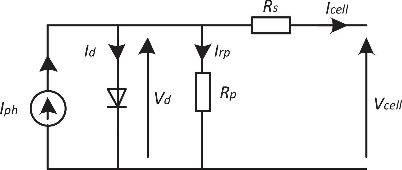
Equivalent PV cell scheme. PV, photovoltaic.
The current Icell can be calculated using the Eq. (1) (Abdessamia et al., 2019; Jesus et al., 2023):
Figure 2 shows the DC–DC converter that optimises power transfer from the PV array to the load. By continuously varying the voltage and current between the PV source and the load (Fares et al., 2024), DC–DC converter ensures that the system operates at the MPP of the PV array (M’hand et al., 2022). For the purpose of optimising power extraction under different environmental circumstances, this procedure known as MPPT is essential (Jaouher et al., 2019).
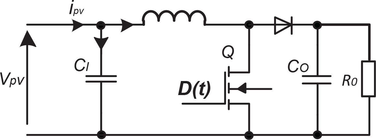
Boost converter circuit.
Eq. (6) represents the fundamental relationship between the mains voltage and the converter duty cycle (Bhukya et al., 2017; Chiheb et al., 2022):
It is essential to consider how the duty cycle and grid voltage interact to enhance the transient response in MPPT management (Shaukat, 2021). We examine a tiny equivalent signal that is comparable to Figure 2 to better analyse the transitory response of the system, as seen in Figure 3.
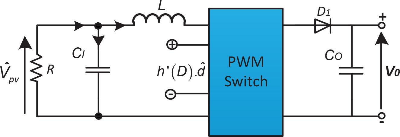
PV output converter circuit: Small-signal model. PV, photovoltaic.
The small-signal duty cycle transfer function at mains voltage is derived based on a specific operating point (Li et al., 2024; Parian and Amiri, 2021). As shown in Figure 3, the Laplace domain equation that relates the mains voltage
The relationship between Vpv and D is shown by h(d), where
The boost converter’s output is denoted by V0. Taking the first derivative of Eq. (9) with respect to duty cycle D, we obtain:
In a steady-state condition, the boost converter output, denoted as V0, is expressed in Eq. (9). This assumes that transient switching effects do not affect h(D) and V0. Consequently, h′(D) = −V0 and Eq. (8) can be reformulated as follows:
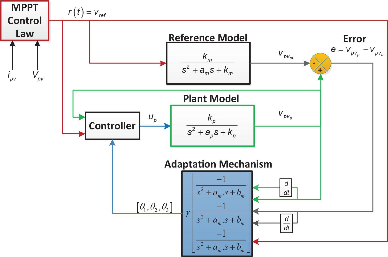
This part represents the MRAC-FUZZY concept, which is designed to increase a solar array’s effectiveness in producing electricity. The comprehensive framework of this control strategy is displayed in Figure 4.
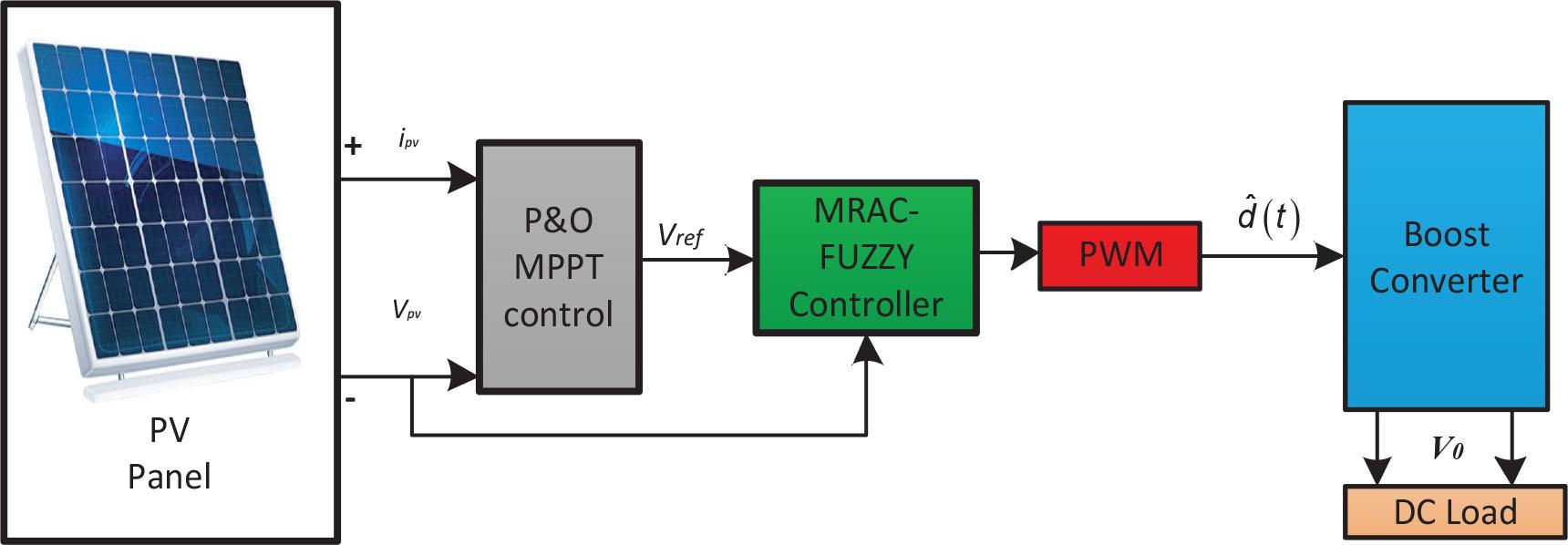
PV system featuring the proposed MPPT control algorithm. MPPT, maximum power point tracking; P&O, perturb and observe; PV, photovoltaic; PWM, Pulse Width Modulation..
The suggested algorithm is organised into two tiers. The starting tier introduces an MPPT control law based on the P&O technique, as illustrated by Algorithm 1. This control block sets a voltage reference (vref) for a given MPP voltage. In the second tier, a novel MRAC-FUZZY MPPT controller has been designed and implemented as shown in Figure 5.
1. Initialize DeltaVref, Pprev, Vprev
2. While system is running do
3. Read current voltage and current from the panel Vpv ,Ipv
4. Calculate the current power Ppv = Vpv *Ipv
5. Calculate the change in voltage:dV=Vpv-Vprev
6. Calculate the change in voltage:dP=Ppv-Pprev
7. if (dP) ~= 0
8. Vref=Vpv
9. else
10. if (dP) > 0
11. if (dV) > 0
12. Decrease reference voltage : Vref = Vprev - deltaVref;
13. else
14. Increase refence voltage : Vref=Vprev + deltaVref;
15. end if
16. else
17. if (dV) > 0
18. Increase refence voltage Vref = Vprev + deltaVref;
19. Else
Block scheme of the suggested MRAC controller. MPPT, maximum power point tracking.
The reference voltage and the array voltage are the only two inputs of the recently created adaptive MPPT controller. As seen in Figure 5, the proposed MRAC controller contains a plant model, a reference model and an adaptation gain (γ).
The aim of MRAC is to match the output of a plant with that of a reference model using a parameter (γ). To implement MRAC effectively, the first step is to choose a suitable reference model. Subsequently, a controller must be designed to minimise the error (e) between the outputs of the reference model and the plant (Jagadeshwar and Das, 2022). A key adaptive technique in this context is the Massachusetts Institute of Technology (MIT) rule, which utilises a gradient-based method. Developed in the 1960s at MIT for aerospace applications (Madhavan and Ansari, 2022; Mahbouba et al., 2022), the MRAC controller enhances this approach by adjusting adaptation laws to reduce the difference between the reference model’s output and the actual system output.
Second-order systems do not benefit from standard MRAC feedback. This section outlines the control law for second order systems and details the extension of MRAC-FUZZY from first to second order. The following equation defines the plant model:
The transfer function of the plant model is given by:
The relationship between the output
Applying the MIT rule, the cost function is defined as:
Eq. (18) is used in the proposed algorithm as the controller. The controller structure shown in Figure 5 is designed to achieve the desired control objectives. For a bounded reference input, the control law Up is defined as:
Using Eqs. (15) and (20), we can obtain:
Using Laplace transformation, the Eq. (20) becomes
The error e given by Eq. (17), can be rewritten as follows:
The sensitivity derivatives
Assuming that
The adaptation gain γ significantly affects the system’s performance and is usually determined through heuristic methods (Mahbouba et al., 2022b; Tahmid et al., 2023). In the proposed algorithm, to ensure optimal performance, the value of γ is determined using a FLC. As previously mentioned, the fuzzy controller requires one output and two inputs as depicted in Figure 6.
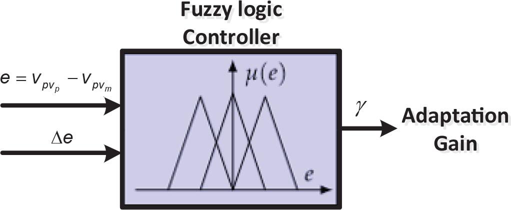
Structure of the FL γ adaptation. FL, fuzzy logic.
Each fuzzy controller variable universe of discourse (e, ∆e) is divided into five triangular membership functions fuzzy sets, leading to a total of 25 inference rules. The fuzzification approach employed is the Max–Min method (Mamdani) (Mazen et al., 2021).
Table 1 displays the inference rules for determining the adaptation gain in a matrix format, often referred to as the ‘Inference Matrix’ (Rai and Rahi, 2022).
For example, the interpretation of the rule corresponding to the red cell in Table 1 is: if the error is negative big (NB) and the variation of error is Zero (ZO), the value of the adaptation gain is Small (S) (Hichem et al., 2019; Pankaj and Rajiv, 2021). These rules can be used to create a 3D control surface, which is shown in Figure 7.
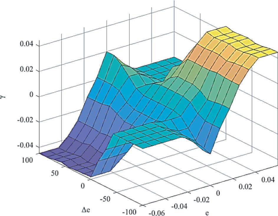
Control surface of the fuzzy controller.
Various simulation tests are performed using MATLAB-Simulink. Tables 2 and 3 present the panel, the boost converter parameters and the coefficients for the developed technique. To assess the efficacy of our methodology, a comparative study is performed with traditional MPPT control approaches, including P&O, P&O-PI, and across diverse temperature and radiation conditions.
Fuzzy control rules for calculating.
| E | ||||||
|---|---|---|---|---|---|---|
| γ | NB | NS | ZO | PS | PB | |
| ∆e | NB | Z | Z | B | B | B |
| NS | Z | Z | S | S | S | |
| ZO | S | Z | Z | Z | S | |
| PS | S | S | S | Z | Z | |
| PB | B | B | B | Z | Z | |
NB, negative big; NS, Negative Small; PB, Positif Big; PS, Postif Small; ZO, zero.
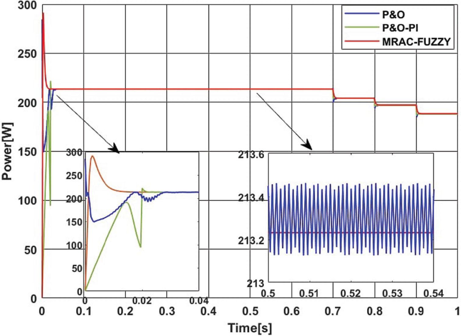
Figure 8 illustrates the variation in the radiation signal. The selected signals consist of three states, with the temperature remaining constant at 25°C throughout the process. Figures 9a and 9b show the PV power and voltage using three different MPPT algorithms (proposed MPPT, P&O and P&O-PI) under conditions of rapidly fluctuating solar radiation. The results of the three tracking techniques are matched, but the proposed MRAC-FUZZY MPPT algorithm improves the system settling time, overshoot and the efficiency as shown in the zoomed region in Figures 9 and 10 and Table 4.
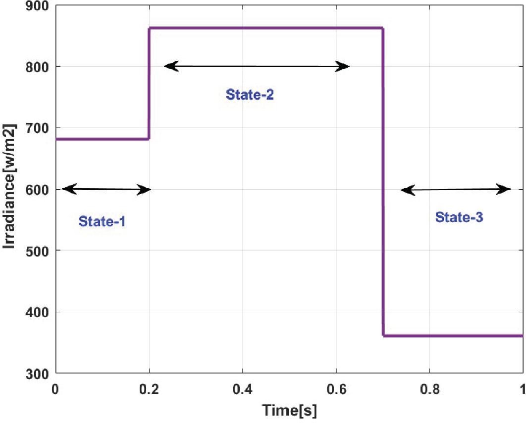
Irradiation pattern profile.
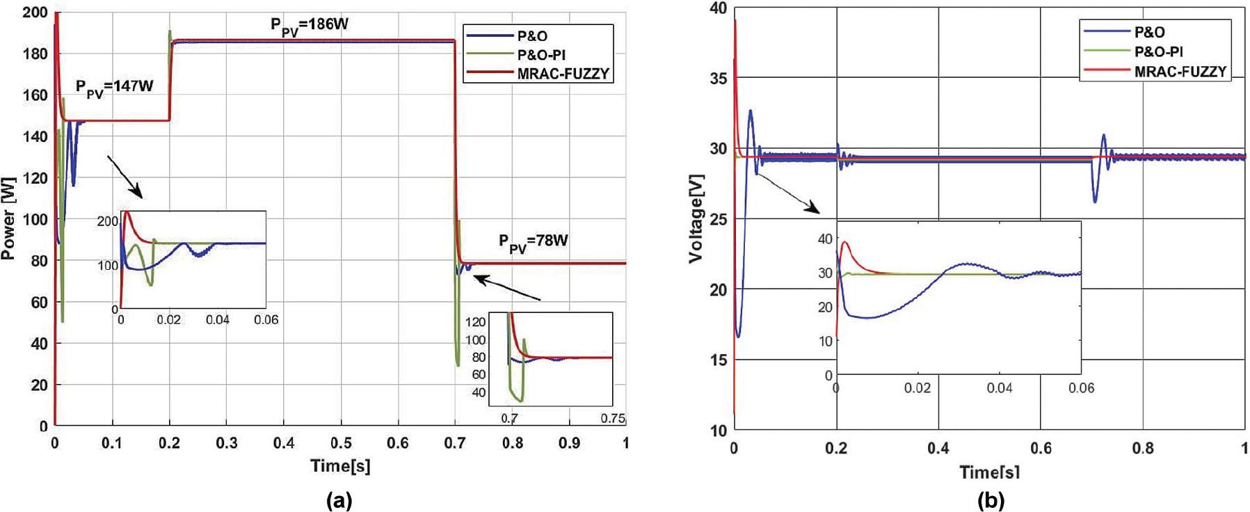
Simulation results for three MPPT controllers for different radiation and a fixed temperature. MPPT, maximum power point tracking; P&O, perturb and observe. (a) Power, (b) Voltage.
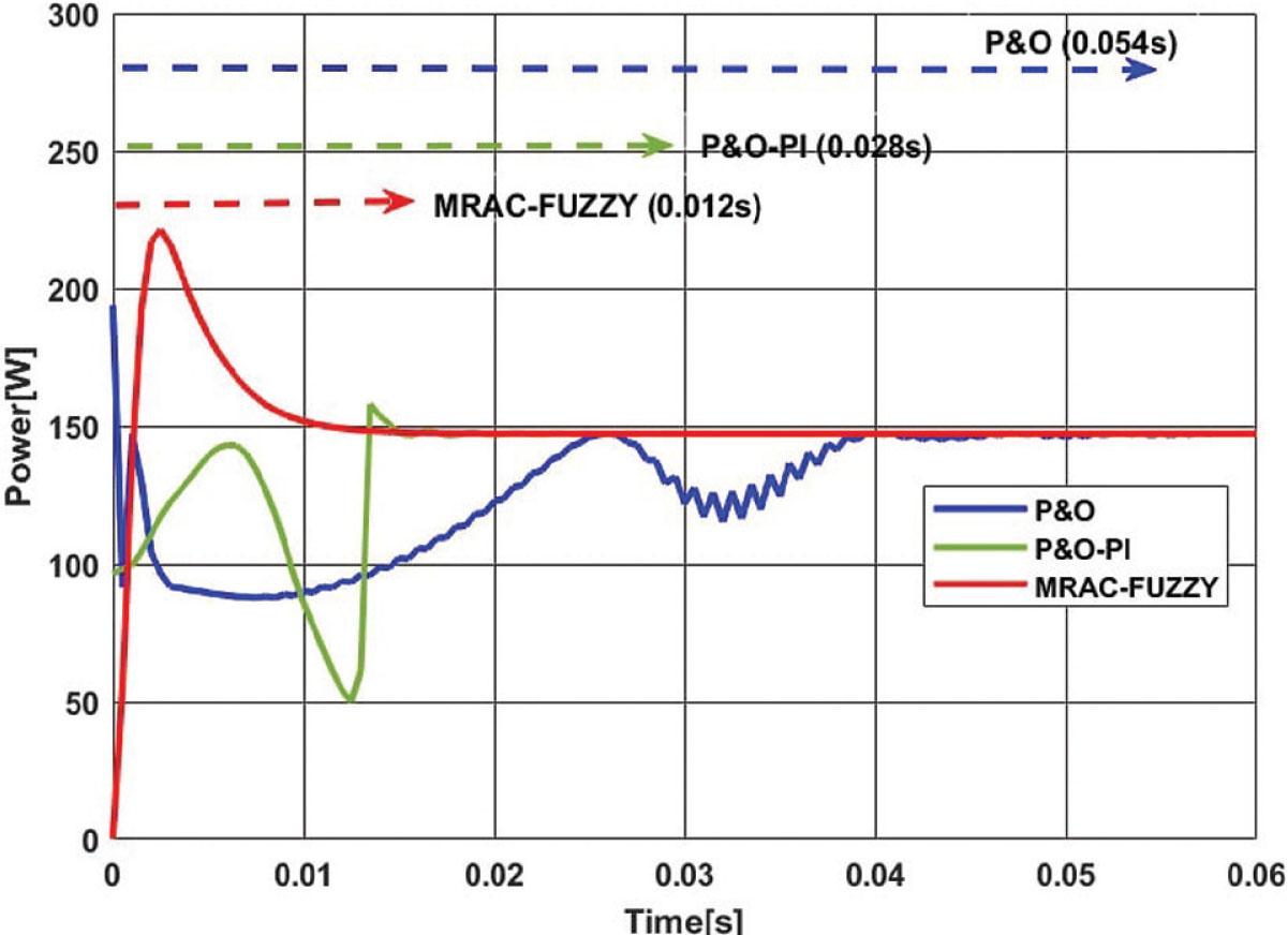
MPPT speed with varying irradiance and constant temperature. MPPT, maximum power point tracking; P&O, perturb and observe.
Figures 9 and 10 illustrate that the P&O technique takes the longest time to reach the MPP, approximately 0.054 s. This is followed by the P&O-PI technique at 0.028 s. By contrast, the proposed technique reaches the MPP in just 0.0012 s. Additionally, both the P&O-PI and the P&O methods display significant ripples around the MPP. From the obtained results, it is clear that the proposed MRAC-FUZZY-based MPPT control exhibits the shortest response time, the lowest ripple and energy losses and the highest efficiency.
Simulation parameters.
| PV model parameters | Value | DC–DC boost parameters | Value |
|---|---|---|---|
| Maximum power (PMPP) | 213.15 W | CI | 100 µF |
| Maximum current (IMPP) | 7.35 | VIN | 56.6–60.3 V |
| Maximum voltage (VMPP) | 29 V | L | 2 mH |
| Short-circuit current (Isc) | 7.84 A | R0 | 20 Ω |
| Open-circuit voltage (Voc) | 36.3 V | CO | 100 µF |
| Number of parallel modules | 2 | V0 | 112.5–129.1 V |
| PV cell Rpe | 313.4 Ω | ||
| Number of series module | 2 | ||
| PV cell Rse | 0.39 Ω | ||
| Cells per module | 60 | ||
| Ri | 25 Ω |
PV, photovoltaic.
MRAC-FUZZY control parameters.
| MRAC_FUZZY parameters | Value |
|---|---|
| ap = 1/(RxCI) | 400 (rad/s) |
| am | 8.17 × 10³ (rad/s) |
| bp = bm 1/L × CI | 1.67 × 10⁷ (rad/s)2 |
| kp = V0 /L × CI | 6.45 × 10⁸ V (rad/s)2 |
| Simulation step time (Ts) | 1 µs |
| Switching frequency (fs) | 20 kHz |
| Km | 5.75 × 10⁸ V (rad/s)2 |
To demonstrate the efficacy of the proposed MPPT algorithm, various performance criteria, including response time, ripples, energy losses and efficiency under three different irradiation conditions, are calculated and presented in Table 4. The obtained simulation data highlight that the novel control algorithm outperforms conventional MPPT control methods, particularly during sudden changes in radiation conditions. Indeed, the proposed MPPT algorithm based on MRAC-FUZZY technique is characterised by its rapid convergence to the MPP during the experimental validation phase, demonstrating significantly reduced oscillations in contrast to conventional algorithms. Ultimately, the tracking efficiency of the PV system has been improved compared to other MPPT algorithms as listed in Table 4. Therefore, the proposed MPPT algorithm improved the system average efficiency in case of varying irradiance with a constant temperature from 95.18% for the P&O algorithm and from 95.83% for the P&O-PI algorithm to 99.96% for the MRAC-FUZZY-based MPPT algorithm.
The three MPPT control approaches were simulated using two different temperature profiles and constant irradiation, as illustrated in Figure 11. Figures 12 and 13 shows the PV output-power and voltage using the proposed MRACFUZZY MPPT, conventional P&O and classical P&O-PI-based MPPT algorithms. The findings from the three tracking techniques are consistent with one another. However, the MRAC-FUZZY-based MPPT algorithm proposed in this study demonstrates improvements in system settling time, overshoot and efficiency, as shown in Figure 13 and the data presented in Table 5. The proposed MRAC-FUZZY-based MPPT algorithm improved the system energy losses in case of varying temperature with constant irradiation from 3.13% for the P&O algorithm and from 1.46% for the P&O-PI algorithm to 0.0005% for the proposed MPPT algorithm.
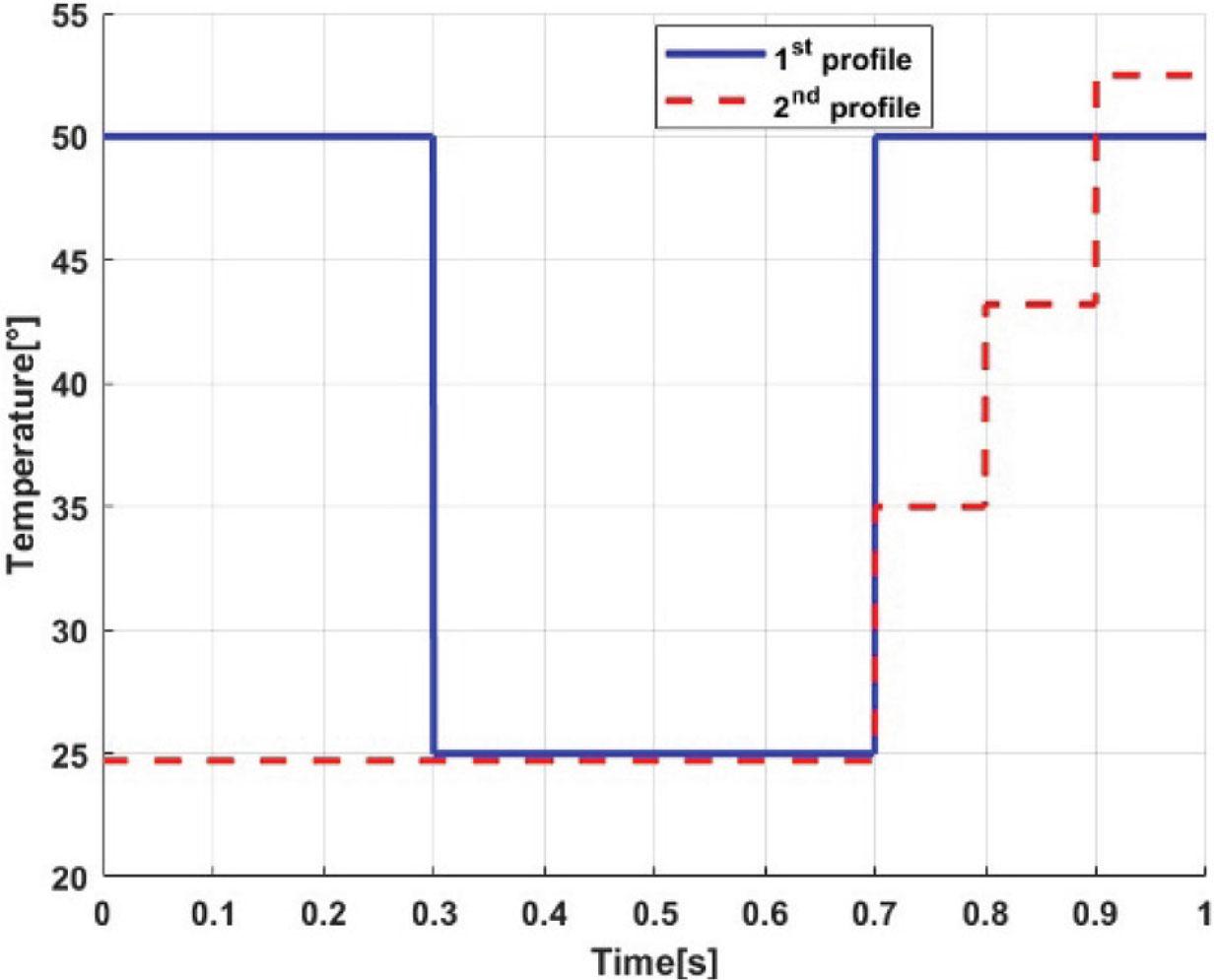
Temperature profile (Pattern 1- and Pattern 2 --).
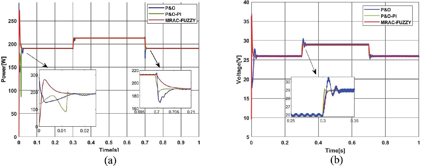
Performance of three MPPT controllers with variable temperature and constant irradiation (Pattern 1). MPPT, maximum power point tracking; P&O, perturb and observe. (a) Power, (b) Voltage.
Three MPPT controllers performing at different temperatures and constant irradiation (Pattern 2). MPPT, maximum power point tracking; P&O, perturb and observe.
Performance comparison of the three algorithms
| MPPT techniques | State-1 | State-2 | State-3 |
|---|---|---|---|
| Response time (s) | |||
| P&O | 0.054 | 0.051 | 0.03 |
| P&O-PI | 0.028 | 0.034 | 0.022 |
| MRAC_FUZZY | 0.012 | 0.013 | 0.01 |
| Ripples (W) | |||
| P&O | 0.957 | 0.2 | 0.21 |
| P&O-PI | 0.55 | 0.12 | 0.1 |
| MRAC_FUZZY | 0.0002 | 0.0001 | 0.0001 |
| Energy losses (%) | |||
| P&O | 3.2 | 2.1 | 4.3 |
| P&O-PI | 1.4 | 1.43 | 3.21 |
| MRAC_FUZZY | 0.0002 | 0.0001 | 0.0004 |
| Efficiency (%) | |||
| P&O | 95.2 | 96 | 94.34 |
| P&O-PI | 96.21 | 96.02 | 95.27 |
| MRAC_FUZZY | 99.96 | 99.98 | 99.94 |
| Average steady state power(W) | |||
| P&O | 147.16 | 184.92 | 78.244 |
| P&O-PI | 147.17 | 185.997 | 78.297 |
| MRAC_FUZZY | 147.22 | 186.266 | 78.36 |
MPPT, maximum power point tracking; P&O, perturb and observe.
The obtained results show that the MRAC-FUZZY MPPT controller has improved the MPPT performance, including good monitoring of the MPP with the absence of remarkable oscillations around the MPP. Conversely, the other MPPT controllers demonstrate delays in reaching the MPP. The MRAC-FUZZY controller achieves the MPP in 0.012 s. It is roughly four times quicker than P&O and twice as quickly as P&O-PI.
Performance comparison of three MPPT algorithms
| MPPT techniques | P&O | P&O-PI | MRAC-FUZZY |
|---|---|---|---|
| Response time (s) | 0.054 | 0.028 | 0.012 |
| Ripple (W) | 0.33 | 0.12 | 0.0001 |
| Energy loss (%) | 3.13 | 1.45 | 0.0005 |
| Efficiency (%) | 95.2 | 96.21 | 99.94 |
MPPT, maximum power point tracking; MRAC-FUZZY, Model Reference Adaptive Controller-FUZZY; P&O, perturb and observe; P&O-PI, Perturb and Observe-Proportional Integral.
An analysis comparing the suggested approach to other methods
| Performance parameters | Adaptive MPPT controller (Saibal et al. (2022)) | ANFIS-TRSMC (Mbarki et al. (2022)) | (PSO) (Ersalina et al. (2023)) | (GWO)-PID (Jesus et al. (2023)) | Proposed MPPT |
|---|---|---|---|---|---|
| Tracking time | 0.0036 | 0.04 | 0.012 | 0.018 | 0.011 |
| Oscillations at MPP | Low | Medium | Medium | No | No |
| Complexity | Medium | Medium | Medium | Medium | Low |
| Efficiency (%) | 97.69 | 98.9 | 96.96 | 98.50 | 99.98 |
GWO-PID, Grey Wolf Optimization-Proportional Integral Derivative; MPP, maximum power point; MPPT, maximum power point tracking; PSO, particle swarm optimization.
The MRAC-FUZZY algorithm improves the system’s average efficiency from 95.2% with the P&O and P&O-PI, respectively, to an impressive 99.98%. Furthermore, the proposed MRAC-FUZZY algorithm demonstrates exceptional accuracy in tracking maximum power despite climatic fluctuations, with minimal oscillation around the MPP. This sets it apart from other control methods. The zoomed-in views of Figures 9 and 12 clearly show significant improvements compared to the results achieved with the P&O and P&O-PI MPPT algorithms. These enhancements are detailed below:
- ✓
The tracking time is improved compared to other used algorithms in this work.
- ✓
The power ripple has been greatly reduced.
In comparison to other recent studies presented in Table 6, the PV system’s tracking efficiency has ultimately been improved by 3.02%, 2.29%, 1.48% and 1.08% compared with the previous findings by Ersalina et al. (2023), Saibal et al. (2022), Jesus et al. (2023) and Mbarki et al. (2022).
To boost the efficiency of PV systems, a novel MPPT algorithm based on fuzzy MRAC has been developed. This innovative algorithm combines the robust capabilities of MRAC, adapts at handling non-linear systems, with the heuristic adaptability of FL to set the adaptation gain. The behaviour of the system for MPPT was simulated in the MATLAB/Simulink environment. A comparative analysis was performed against conventional algorithms: P&O and P&O-PI assessing various factors like dynamic response time, ripple reduction and overall efficiency. The simulation results confirmed the new controller’s remarkable efficiency, with a considerable reduction in response time (0.012 s to reach the MPP). It is about four times quicker than P&O and twice as quick as P&O-PI, achieving an efficiency of up to 99.98%. Additionally, the proposed MRAC-FUZZY-based MPPT algorithm ensures precise MPPT without any ripple. In the forthcoming study, we will concentrate on performing a thorough analysis to identify the parameters of the new MRAC-FUZZY-based MPPT algorithm presented in this paper. The objective is to efficiently modify the suggested algorithm’s learning prototype to react to partial shading scenarios and to implement it for PV pumping systems, as well as to explore the application of a hybrid control approach based on the MRAC-Fuzzy2 algorithm.