In recent years, China has strongly supported green and low-carbon industries. Optimizing energy supply and increasing green products are now urgent for sustainable economic development. As a substitute for fossil energy, lithium-ion batteries are widely used in energy storage, transportation, electronic communication equipment, and other industries [1, 2]. As an excellent cathode material for lithium-ion batteries, the Ni-Co-Mn (NCM) ternary cathode material has the advantages of high energy density, high safety, and good cycle stability [3, 4]. It can greatly improve the storage capacity of lithium-ion batteries. The NCM ternary precursor is one of the main raw materials for NCM cathode materials and is composed of three important elements: Mn, Ni, and Co. The contents of Mn, Co, and Ni have a great impact on the energy density, specific capacity, cycle performance, safety performance, and cost of lithium batteries [5, 6]. To balance the performance and cost of the battery, the contents of Mn, Co, and Ni need to be strictly controlled during the production process. Currently, the commonly used methods to detect element content in NCM ternary precursors are mainly inductively coupled plasma (ICP), atomic absorption spectrometry (AAS), chemical analysis, etc. Although these methods are very accurate [7, 8], they have problems such as the high cost of the analysis process, cumbersome sample preparation [9], and the need for a large amount of chemical reagents [10, 11]. Because the energy-dispersive X-ray fluorescence (EDXRF) technique has the advantages of simultaneous analysis of multiple elements, simple sample preparation, simple operation, fast analysis speed, economical, and non-destructiveness [12, 13], this technique is used to detect and analyze the content of Mn, Co, and Ni of NCM ternary precursor.
When using EDXRF to quantitatively analyze the element content of NCM ternary precursor, the analysis results are easily affected by the absorption-enhancement effect between elements in the sample [14]. This effect is particularly obvious when there is a large difference in concentration between the test sample and the standard samples. That will cause a non-negligible deviation in the analysis results. To solve this problem, researchers proposed to use the matrix dilution method [15, 16] and the standard addition method [17, 18]. The standard addition method adds standard samples to the test sample and creates a calibration curve for quantitative analysis. However, this method does not correct for the inter-element absorption-enhancement effects. Therefore, it is not used in this study. The matrix dilution method can make the matrix composition of the test sample approximately consistent with the standard samples. Then interference of the matrix effect on the analyzed elements can be reduced effectively [15, 16]. At the same time, the accuracy of the analysis results is also improved. However, due to the presence of matrix effects [19], the relationship between the characteristic X-ray intensity and the dilution factor is not linear. So, the sample needs to be diluted step by step to determine the appropriate dilution factor. The process of multiple dilutions and measurements is relatively time-consuming and labor-intensive when compared to a single dilution step while attempting to find out the dilution factor in advance. If a method can be used to calculate the intensity of characteristic X-rays in a diluted sample, the appropriate dilution factor can be quickly determined. This saves time and effort, especially in scenarios that require multiple dilutions.
Based on the traditional matrix dilution method, this study proposes an improved matrix dilution method. This method establishes a functional relationship model between the dilution factor and the characteristic X-ray intensity. If the concentration of the test sample is much higher than that of the standard samples, the diluted characteristic X-ray intensity can be calculated using this functional relationship model. Then, the quantitative analysis can be performed using the calibration curve. There is no need to dilute the sample further or prepare high-concentration standard samples. The innovation of this method lies in its ability to perform quantitative analysis on all samples in the same series (samples with the same elements and proportions of target elements but different concentrations), using the same set of standard samples. This method can theoretically be used for quantitative analysis of all samples regardless of concentration differences. In contrast with the traditional matrix dilution method, this approach requires the dilution of only one test sample. It eliminates the need to dilute each sample individually, thus saving time and enabling quantitative analysis.
Based on the theoretical calculation formula of the characteristic X-ray intensity, a functional relationship model between the dilution factor and the characteristic X-ray intensity of the analyzed element was established. During the dilution process, matrix composition and element concentration changes with the dilution factor. This model takes into account the variation of matrix composition and element concentration.
To simplify the calculation process, the continuous spectrum of primary radiation generated by the X-ray tube was regarded as a certain monochromatic ray, and its intensity is shown in Eq. (1) [16]:
The primary radiation generated by the X-ray tube excited the elements, and the characteristic X-ray intensity produced is described by Eq. (2) [15, 16, 20]:
The element concentration in the test samples was much higher than that in the standard samples. Therefore, it was necessary to dilute the test samples. Deionized water was used to dilute the NCM ternary precursor solution in a certain proportion to obtain the test samples. Assume that 1 mL of the test sample consists of a (a is a variable not >1 mL) of NCM ternary precursor solution, and 1–a mL of deionized water, then the dilution factor of the test sample is 1/a. The density of deionized water was 1 g/cm3. The characteristic X-ray intensity generated by element i in the test sample can be described by Eq. (3):
In the Eq. (3), the meanings of D, K, and x are as follows:
In Eq. (3), Ii,x represents the net intensity of the characteristic X-rays of element i in the diluted solution with dilution factor x, IλP is the intensity of primary radiation with an equivalent wavelength of λP, Pi is the excitation factor, Ci is the concentration (mass fraction) of the element i, and μi,λP is the mass absorption coefficient of the element i for the primary radiation. For the same fluorescence spectrometer, the same unknown sample, and the same dilution factor, K and D are constant. In Eq. (4), A is the geometric factor of the spectrometer, μm,λP and μm,λi are the mass absorption coefficients of the matrix for the primary radiation and the characteristic X-ray of element i, respectively. In Eq. (5), μw,λP and μw,λi are the mass absorption coefficients of water for primary radiation and the characteristic X-ray of element i respectively, ρm denotes the density of the test sample. In Eq. (6), x is the volume dilution factor, a represents the volume of the NCM ternary precursor solution in a 1 mL test sample.
Transforming Eq. (3) yielded Eq. (7). Equation (7) reflects the functional relationship between the dilution factor x and the characteristic X-ray intensity. Accordingly, the net intensity of the characteristic X-rays of the elements at different dilution factors can be calculated using Eq. (7), followed by quantitative analysis.
In Eq. (7), the meanings of k, and b are as follows:
In Eq. (7), Ii,x represents the net intensity of the characteristic X-rays of element i in the diluted solution. For the same fluorescence spectrometer, k and b are constants. Other parameters are the same as in Eqs. (3)–(6). Since the parameters such as IλP, A, and ρm were difficult to obtain, the parameters k and b were obtained by fitting. Then Eq. (7) can be used to calculate the dilution factor based on characteristic X-ray intensity, avoiding step-by-step dilution. It can also determine X-ray intensity from the dilution factor, reducing sample dilution.
After calculating the characteristic X-ray intensity of the element using Eq. (7), quantitative analysis was performed in combination with the calibration curve. The calibration curve represents the linear relationship between the concentration of each element and its characteristic peak area, as shown in Eq. (10) [15]:
The improved matrix dilution method involved diluting the same test sample several times using different dilution ratios and measuring it, establishing a curve based on Eq. (7). Thereafter, the resulting curve was used to calculate the characteristic X-ray intensity for quantitative analysis. Afterward, the curve was used directly without further sample dilution. This experiment primarily verified the feasibility of Eq. (7).
The test sample was NCM ternary precursor solution, sourced from a battery materials manufacturing company in Sichuan, China. The national standard solution of Mn, Co, and Ni was sourced from the National Nonferrous Metals and Electronic Materials Analysis and Testing Center of China. Deionized water was sourced from Xizhimeng Trading Co., Ltd. of China, with conductivity <0.1 μs/cm.
Energy spectrum measurements were performed using a CIT-3000SYE EDXRF spectrometer, from Xinxianda Measurement and Control Technology Co., Ltd., Chengdu City, Sichuan Province, China. The detector of the spectrometer was a silicon drift detector, and the energy resolution was 125 eV at 5.9 keV. The anode target of the X-ray tube was a silver target, the tube voltage was 49 kV, and the tube current was 196.1 μA. All samples' acquisition time was 3 min.
Seven test samples with different dilution factors were prepared. NCM ternary precursor solution was diluted with deionized water in a 10 mL volumetric flask, according to the dilution factors of 1, 2, 10, 20, 50, 100, and 200. Thereafter, 5 mL of the solution was aspirated from the volumetric flask into seven polyethylene sample vials using a pipette, labeled S1–S7.
Nine standard samples for quantitative analysis, and six standard samples for calculating the limits of quantification and detection were prepared. 1000 μg/mL national standard solution of Mn, Co, and Ni and deionized water were used to prepare the samples. They were transferred into a 10 mL volumetric flask, according to the concentrations of Mn, Co, and Ni listed in Table 1. A pipette was then used to draw 5 mL of the sample solution from the volumetric flask, and transferred it into a polyethylene sample cup to make nine standard samples (as shown in Table 1).
Standard samples information
| Standard sample no. | Mn concentration (mg/mL) | Co concentration (mg/mL) | Ni concentration (mg/mL) |
|---|---|---|---|
| SS1 | 100.0 | 100.0 | 100.0 |
| SS2 | 300.0 | 300.0 | 300.0 |
| SS3 | 325.0 | 140.0 | 360.0 |
| SS4 | 120.0 | 130.0 | 330.0 |
| SS5 | 240.0 | 260.0 | 500.0 |
| SS6 | 180.0 | 150.0 | 350.0 |
| SS7 | 160.0 | 130.0 | 330.0 |
| SS8 | 140.0 | 110.0 | 310.0 |
| SS9 | 120.0 | 90.0 | 290.0 |
| MnSS1 | 100.0 | 0.0 | 0.0 |
| MnSS2 | 200.0 | 0.0 | 0.0 |
| MnSS3 | 300.0 | 0.0 | 0.0 |
| CoNiSS1 | 0.0 | 100.0 | 100.0 |
| CoNiSS2 | 0.0 | 200.0 | 200.0 |
| CoNiSS3 | 0.0 | 300.0 | 300.0 |
The energy of the Kα line of Co (6.93 keV) and Ni (7.47 keV) is slightly greater than the K-absorption edge of Mn (6.54 keV). The characteristic X-rays of Co and Ni can indeed excite the K-shell electrons of Mn, leading to enhanced emission of Mn's K-series characteristic X-rays [19]. To determine the limit of detection (LOD) and quantification of Mn, and reduce the impact of Co and Ni on Mn, standard samples (MnSS1–MnSS3) were prepared using Mn standard solution and deionized water. In the label ‘MnSS3’, the ‘Mn’ represents Mn, the first ‘S’ represents ‘Standard’, the second ‘S’ represents ‘Sample’, and ‘3’ represents the index. The mutual influence between the characteristic X-rays of Co and Ni was minimal. Therefore, to determine the LOD and quantification of Co and Ni, standard samples (CoNiSS1–CoNiSS3) were prepared using Co and Ni standard solutions (as shown in Table 1).
The concentration information in Table 1 was obtained through theoretical calculations. The volume of each sample was 5 mL, and the samples were used to draw the calibration curves. Mn (Kα, 5.90 keV) and Pb (Lα, 10.55 keV) standard samples were used for energy line calibration.
The spectrums of the diluted NCM ternary precursor solution (samples S1–S7) were measured. The arithmetic average method with a smoothing width of nine points was used to smooth spectra. Gaussian fitting was performed on the characteristic peaks of the analyzed elements, and the trapezoidal method was used to subtract the background. The net peak area of the analysis line of the analyzed elements was calculated, and then the dilution factor-characteristic X-ray intensity curves were established according to Eq. (7).
Afterward, the spectrums of the standard samples (samples SS1–SS9) were measured, and the processing procedure was the same as that for the spectrum of the test sample. The calibration curves were established according to Eq. (10).
Thereafter, the spectrums of standard samples (MnSS1–MnSS3, CoNiSS1–CoNiSS3) were measured. The processing procedure was the same as that for the spectrum of the test sample. According to the spectrums, calibration curves were established for the limits of detection and quantification.
Software CIT-3000SYB (version 3.0A, manufactured by Xinxianda Measurement and Control Technology Co., Ltd. located in Chengdu City, Sichuan Province, China) was used to collect the energy spectrums. Each sample was measured three times.
Quantitative analysis was performed using the improved matrix dilution method. Based on the established dilution factor-characteristic X-ray intensity curves, the characteristic X-ray intensity of the test samples was calculated. The elemental content was then calculated according to Eq. (10). Secondly, to compare the accuracy of the method, quantitative analysis was performed using the traditional matrix dilution method. Based on the measured values of the characteristic X-ray intensity, the elemental content of the test samples was calculated using the calibration curves. Thirdly, statistical analysis of the data was performed. Error bars representing the uncertainty of the measured data were expressed as ‘mean ± SD’ in the figures. A two-tailed t-test was used to check if the calculation results of the two methods were consistent.
According to the calculation formula of the International Union of Pure and Applied Chemistry (IUPAC), the LOD refers to the lowest concentration of an element that can be detected, and the limit of quantification (LOQ) refers to the lowest detectable concentration during quantitative analysis. Its definition is shown in Eqs. (11) and (12) [16, 21]:
Low-concentration standard samples of the Mn, Co, and Ni (samples MnSS1, MnSS2, MnSS3, CoNiSS1, CoNiSS2, CoNiSS3) were measured, and a calibration curve was established for each element. Then LOD and LOQ were calculated according to Eqs. (11) and (12).
The energy spectrum measurement of sample S6 was repeated 10 times, and then the precision of each element was calculated according to Eq. (13) [16]:
Quantitative analysis errors mainly arise from operational errors in sample preparation and statistical errors in spectral intensity, among others. The following describes the method used in this study to evaluate the errors in the results of the quantitative analysis. The mole percentages Ci,cal of the three elements were compared with the standard results Ci,S obtained by chemical analysis methods. The relative error RE(i) [22] of element i was calculated according to Eq. (14). The RE of Mn, Co, and Ni were averaged to obtain the average relative error MRE using Eq. (15). The quantitative analysis results of the test samples under the two methods were discussed.
The energy spectrum of the NCM ternary precursor solution (sample S1) measured by the X-ray fluorescence spectrometer is shown as black data points in Fig. 1. To minimize the effect of statistical fluctuations on the spectral peaks, Gaussian fitting was applied to the peaks to estimate the net intensity of the characteristic X-rays. The fitting curves are illustrated by the red curves in Fig. 1.
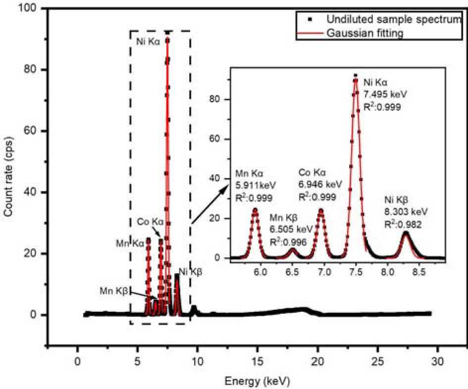
Sample energy spectrum of the test sample S1 (undiluted NCM ternary precursor solution).
As shown in Fig. 1, the Kβ peak (7.65 keV) of the Co element was not observed between the Kα peak (6.92 keV) of Co and the Kβ peak (8.27 keV) of Ni. This was because the energy of the Kβ line of Co is close to that of the Kα line (7.47 keV) of Ni. The silicon drift detector's energy resolution was insufficient to distinguish between them. That resulted in the overlap of the Kα peak of Ni with the Kβ peak of Co [23]. Additionally, the energy of Kα characteristic X-ray of trace Fe (6.40 keV) in sample S1 is close to that of Kβ characteristic X-ray of Mn (6.50 keV), which also led to a slight increase in the intensity of the Kβ characteristic X-ray of Mn. From the energy of the K-series characteristic X-rays and K-absorption edges of Mn, Co, and Ni, it can be inferred that there was an absorption-enhancement effect among these elements [19]. That is, Co and Ni enhanced the intensity of the K-series characteristic X-rays of Mn, and the Kβ characteristic X-ray of Ni enhanced the intensity of the K-series characteristic X-rays of Co. Besides that, the Kβ line of Mn was weak and interfered with Fe, and the background interfered with the Kβ line of Ni. Therefore, the Kα lines of Mn, Co, and Ni were chosen as the analytical lines.
The results are shown in Fig. 2. The linear fitting coefficients of determination of the calibration curves of Mn, Co, and Ni elements were 0.956, 0.981, and 0.997, respectively. That indicates that the net peak area of element characteristic peaks was highly linearly related to the element content. However, due to the relatively high content of Ni, the Kα characteristic X-ray was less affected by Mn and Co, thereby exhibiting better linearity. At the same time, since the Mn content was low, the enhancing effect of Co and Ni was relatively significant, resulting in a lower linearity of the calibration curve.
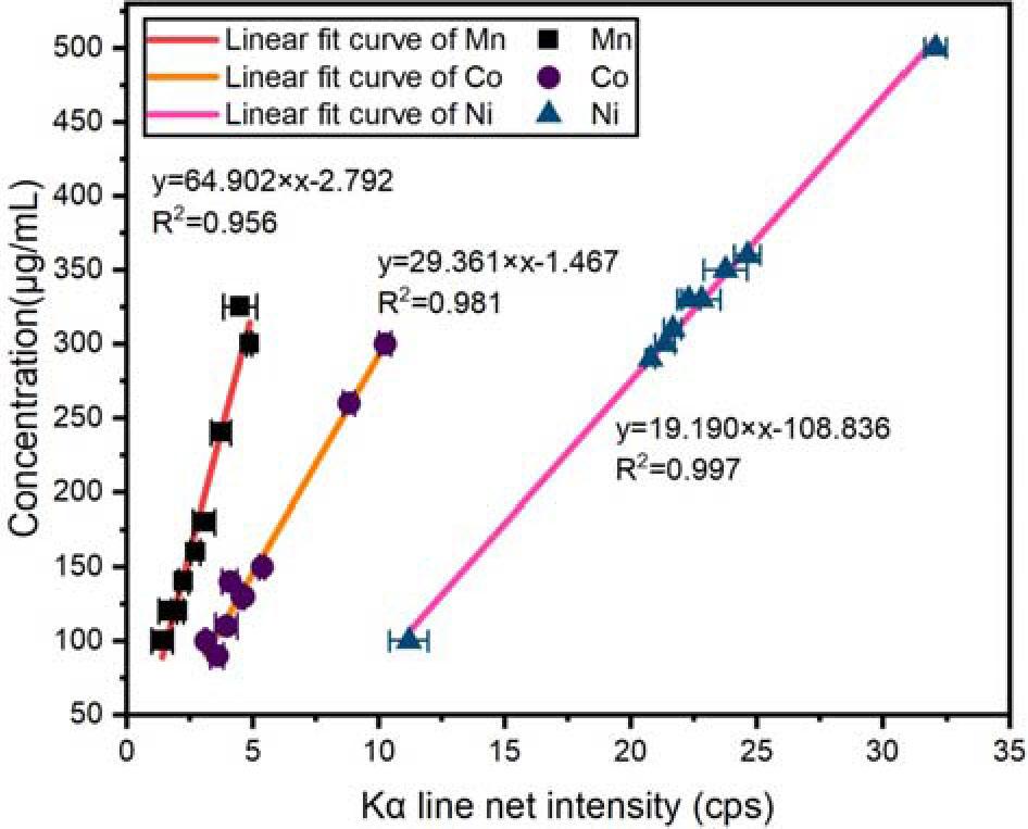
Mn, Co, and Ni calibration curves. The scatter points represent the elements of the standard samples SS1–SS9, and the straight lines are fitted curves. The data provided are in the form of mean ± SD, the number of measurements was three.
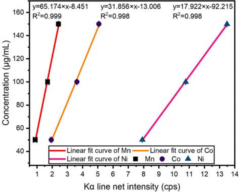
The reciprocal of the Kα characteristic X-ray net peak area of each element was fitted according to Eq. (7), and the dilution factor-characteristic X-ray intensity curves were established. The results are shown in Fig. 3.
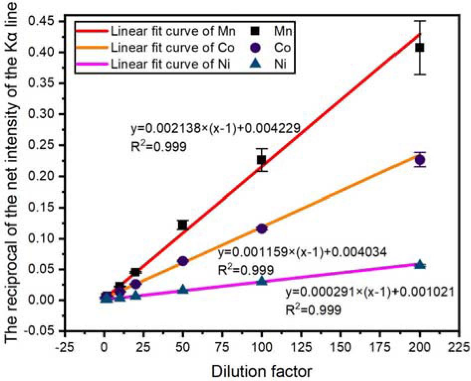
Dilution factor-characteristic X-ray intensity curves of Mn, Co, and Ni. The scatter points represent the elements of the test samples S1–S7. The straight lines are fitted using Eq. (7). The data provided are in the form of mean ± SD, and the number of measurements was three.
As shown in Fig. 3, the reciprocal of the characteristic X-ray intensity had a good linear relationship with the dilution factor, the linear fitting coefficients were all 0.999. The results indicate that the inverse of the intensity of characteristic X-rays was proportional to the amount of diluent added. This can be understood from the denominator of Eq. (2). It shows that the intensity of the characteristic X-rays is inversely proportional to the mass absorption coefficient of the matrix. When the diluent was added, only the mass absorption coefficient of the matrix was changed [16] (although the concentration also changed, it was corrected by multiplying by a factor based on the amount of diluent).
The quantitative results of the improved matrix dilution method are shown in Table 2. According to the established calibration curves, quantitative analysis was performed on the measured values of the characteristic X-ray intensity. The results are shown in Table 3. The relative error RE was calculated using Eq. (14), and the mean relative error MRE of Mn, Co, and Ni was calculated using Eq. (15).
The results of the element content in the test samples using the improved matrix dilution method
| Sample no. | Dilution factor | Mn | Co | Ni | MRE (%) | |||
|---|---|---|---|---|---|---|---|---|
| mol (%) | RE (%) | mol (%) | RE (%) | mol (%) | RE (%) | |||
| S1 | 1 | 38.9 | 36.9 | 17.0 | 14.5 | 44.1 | 14.8 | 22.1 |
| S2 | 2 | 35.0 | 23.4 | 18.0 | 9.8 | 47.0 | 9.3 | 14.1 |
| S3 | 10 | 28.7 | 0.9 | 19.5 | 2.2 | 51.9 | 0.2 | 1.1 |
| S4 | 20 | 27.5 | 3.1 | 19.7 | 0.8 | 52.7 | 1.8 | 1.9 |
| S5 | 50 | 27.1 | 4.7 | 20.0 | 0.4 | 52.9 | 2.2 | 2.5 |
| S6 | 100 | 27.4 | 3.6 | 20.1 | 1.2 | 52.5 | 1.3 | 2.0 |
| S7 | 200 | 28.3 | 0.3 | 20.3 | 2.2 | 51.3 | 0.9 | 1.1 |
The results of the element content of the test samples using the traditional matrix dilution method
| Sample no. | Dilution factor | Mn | Co | Ni | MRE (%) | |||
|---|---|---|---|---|---|---|---|---|
| mol (%) | RE (%) | mol (%) | RE (%) | mol (%) | RE (%) | |||
| S1 | 1 | 38.9 | 36.9 | 16.9 | 15.3 | 44.3 | 14.5 | 22.2 |
| S2 | 2 | 35.0 | 23.1 | 18.1 | 9.0 | 46.9 | 9.4 | 13.8 |
| S3 | 10 | 28.8 | 1.3 | 19.4 | 2.4 | 51.8 | 0.0 | 1.2 |
| S4 | 20 | 27.5 | 3.1 | 19.7 | 0.8 | 52.7 | 1.8 | 1.9 |
| S5 | 50 | 26.2 | 7.8 | 20.4 | 2.4 | 53.4 | 3.1 | 4.4 |
| S6 | 100 | 26.8 | 5.5 | 20.6 | 3.6 | 52.5 | 1.4 | 3.5 |
| S7 | 200 | 28.7 | 0.9 | 19.8 | 0.7 | 51.6 | 0.4 | 0.7 |
Comparing the data in Table 2 with that in Table 3, the calculation results of both were basically consistent. A two-tailed t-test was used to determine whether there was a significant difference between the two groups of data, and the null hypothesis was set that there was no difference between the two groups of data, using an alpha value of 0.05. The results of the two-tailed t-test showed that the P-values for the three elements were as follows: 0.43, 0.75, 0.23, and all P-values were >0.05. Therefore, the null hypothesis cannot be rejected, indicating that there was no significant difference between the two methods. For sample S5 (the dilution factor was 50), the difference in the average relative errors between the two was the largest, which was 1.9%. For sample S4 (the dilution factor was 20), the difference in the average relative errors between the two methods was the smallest, which was 0%. Quantitative analysis results show that the average relative errors of sample S7 (the dilution factor was 200) in the two tables were the smallest, 1.1% and 0.7% respectively. This means when dilution of the sample is needed but the appropriate dilution factor is unknown, Eq. (7) can be used to estimate the appropriate dilution factor. It can also be used to estimate the characteristic X-ray intensity when a specific dilution cannot be prepared. This indicates that, theoretically, with this method, other samples in the same series (with the same elements and proportions but different concentrations) do not require further dilution or additional standard samples. The measured characteristic X-ray intensity can be directly used to perform quantitative analysis using Eq. (7) with the calibration curve. Compared to the traditional matrix dilution method, this approach reduces sample preparation and measurement [15]. Note that this method is not applicable if the elements differ or if there are significant differences in element proportions.
When the dilution factor of the test sample was low, the element concentration in the test sample was high. The original matrix composition in the NCM ternary precursor solution had a great impact on the measurement results, and there was also a strong absorption-enhancement effect between the elements. Equation (7) only considered the primary fluorescence generated by the analytical elements and did not account for the secondary fluorescence or higher-order fluorescence. Therefore, the quantitative analysis results had a relatively large error. When the dilution factor was 200, the element concentration was within the concentration range of the standard sample. The original matrix component in the NCM ternary material solution had less influence on the measurement results, so the error was smaller. Although the average error MRE of the test sample S3 was consistent with that of the test sample S7, the error of the mass fraction of the elements analyzed quantitatively was very large. This was due to the characteristic X-ray intensity of sample S3 being far higher than that of the standard samples, and the matrix effect caused significant errors [15, 16, 19]. Therefore, it is not used as the quantitative analysis result.
The calibration curves used to calculate the LOD and quantification are shown in Fig. 4. The limits of detection of Mn, Co, and Ni calculated using Eq. (11) were 5.25 μg/mL, 4.55 μg/mL, and 9.09 μg/mL respectively. The limits of quantification of Mn, Co, and Ni calculated using Eq. (12) were 17.49 μg/mL, 15.17 μg/mL, and 30.30 μg/mL respectively. Due to the higher background of Ni, its detection limit and quantification limit were higher than those of the other two elements. From the results of LOD and LOQ, the elemental concentrations of all samples in this article were higher than the LOQ, meeting the minimum requirements for quantitative analysis [15, 16].
Calibration curves used to calculate the LOD and quantification of Mn, Co, and Ni. The scatter points represent the elements of the standard samples MnSS1– MnSS3 and CoNiSS1–CoNiSS3. The straight lines are fitted curves. The data provided are in the form of mean ± SD, the number of measurements was three.
Precision is an indicator of the repeatability of an experiment. The precision calculation results of Mn, Co, and Ni calculated using Eq. (13) were 26.94 μg/mL, 3.88 μg/mL, and 8.36 μg/mL respectively. Therefore, the precision of this experiment was good, with the Co element having the best precision and the Mn element having the worst precision. This result shows that the statistical fluctuation under experimental conditions was small, the repeatability was good, and the measurement results were relatively reliable [15, 16].
This method can calculate the characteristic X-ray intensity based on the dilution factor, thus avoiding the preparation of some unnecessary samples. However, Eq. (7) can only calculate the intensity of primary fluorescence, meaning that the calculated result's error is partly due to secondary and higher-order fluorescence. The next step of this study is to correct the effect of secondary fluorescence in Eq. (7), improving the accuracy of quantitative analysis of the NCM ternary precursor solution. When x in Eq. (7) is <1, the calculated fluorescence intensity represents the intensity of the sample after concentration. The next step of this study will also verify if Eq. (7) is applicable to concentrated samples. If this is found to be feasible, Eq. (7) can be used to calculate the fluorescence intensity of a substance that does not contain moisture.
Based on the traditional matrix dilution method, this study established dilution factor-characteristic X-ray intensity curves. The minimal quantitative analysis errors of Mn, Co, and Ni were 0.3%, 2.2%, and 0.9% respectively for the improved matrix dilution method, 0.9%, 0.7%, and 0.4% respectively for the traditional matrix dilution method. The largest difference in the average relative errors between the two methods was 1.9%. The calculation results of the two were basically consistent, proving that this method can accurately calculate the characteristic X-ray intensity of elements based on the dilution factor. If the concentration differences between the test samples are significant, but the element ratios are consistent, this method is a good solution.