
1. Introduction
Wind tunnel testing is an essential means for aircraft development and theoretical studies in aerodynamics. Strain gauge balances are critical force transducers in wind tunnel tests [1], used to measure the aerodynamic loads acting on the test models [2],[3],[4],[5],[6],[7],[8], and are highly valued by leading aerodynamic institutions worldwide. A significant body of research has been continuously conducted on balance optimization design [9]-[10], manufacturing technology [11], strain gauge bonding techniques, temperature compensation methods [12]-[13], calibration technologies [14],[15],[16],[17], and experimental applications [18], leading to notable advancements in wind tunnel testing technologies.
Reducing the development cycle and improving the design quality of balances can facilitate rapid progress in advanced aircraft development during the wind tunnel testing phase, thereby enabling precise aerodynamic performance evaluations. Balances, primarily designed within given dimensional constraints and loading conditions, have traditionally focused on selecting suitable component arrangements through optimization techniques to achieve appropriate design sensitivity, along with verifying strength, stiffness, and other key parameters. Neither early calculations based on mechanics of material formulas nor the current mainstream finite element analysis (FEA), grounded in linear elastic mechanics, can accurately predict the comprehensive static calibration (SC) matrix, which characterizes the relationship between balance bridge outputs and measured loads. This limitation poses a disparity when compared to the stringent force measurement demands of wind tunnel tests for advanced aircraft models.
In the traditional balance development mode, the SC matrix and performance specifications of the balance are calibrated [19] only after structural design, fabrication, strain gauge bonding, temperature compensation, and other related processes are complete. During the design phase, the sensitivity coefficients and linear terms of the SC matrix can generally be estimated using linear FEA; however, the non-linear terms cannot be fully captured due to the geometric non-linearity of the balance. Consequently, this traditional approach does not allow for a complete evaluation of the calibration matrix at the design stage. If the balance's performance specifications fail to meet technical requirements, either performance concessions must be made or the balance must be redeveloped, both of which significantly compromise the quality of aerodynamic data or prolong the vehicle development cycle.
This study introduces an innovative virtual calibration (VC) method for balances based on non-linear FEA to address the limitations of the traditional development approach. In this method, non-linear FEA is performed on a high-performance computer to simulate balanced SC loading. By correlating the balance bridge outputs with the applied loads, the VC matrix for the balance is fitted. Since this method enables the VC matrix to be obtained at the design stage, it offers clear advantages for evaluating balance design quality and optimizing balance performance during development — particularly for new-type balances with complex structures.
2. Balance vc method
A. Calibration math model
For a strain gauge balance, the mathematical model can be described by a second-order polynomial function. The general second-order calibration mathematical model is given as follows:
where Fi is the load applied to the i-th component of the balance; ΔUi is the bridge output of the i-th component; αi is the sensitivity coefficient of the i-th component; bi,j is the linear interference coefficient; c1i,j is the quadratic interference coefficient, and c2i,j,k is the cross-product interference coefficient.In actual load measurement, the initial iteration values are calculated as and then substituted into (1) for iterative calculation. This yields the iterative sequence . The iteration terminates when is less than the convergence tolerance δi.
B. VC method
The VC of a balance is determined through numerical simulations of the SC process at the design stage, which involve solid modeling, simulation analysis, strain gauge bridge circuit processing, and VC data processing. The solid modeling of the balance is carried out using 3D modeling software, and the simulation analysis is performed using FEA software. The simulation analysis process includes importing a 3D model into FEA software, setting material properties, applying boundary constraints, loads, meshing, and solving. It should be noted that the Large Deflection effect and the Newton-Raphson option are enabled when solving the non-linear equations to realize the VC of the balance.
A one-piece balance is generally a complex structure made of high-strength steel that exhibits complex non-linear behavior under multidimensional loading. The weaker the balance stiffness, the greater the non-linearity. For the VC method, the incremental equations are employed in non-linear FEA. Therefore, it is recommended that each load step include 3 sub-steps under non-linear conditions, since an excessive number of load steps may consume significant computational resources.
After the simulations are complete, the strains at the strain gauge bonding positions are extracted from the simulation results. According to the Wheatstone full-bridge measurement principle, the strains produced by four strain gauges R1 to R4 (see Fig. 1) are denoted as ε1 to ε4. The output of the Wheatstone bridge is given as follows:
where ΔUi is the bridge output; k is the nominal gauge factor of the strain gauges; ε1 to ε4 are the strains derived from the corresponding strain gauges R1 to R4 of the Wheatstone full-bridge (see Fig. 1); and Ue is the supply voltage.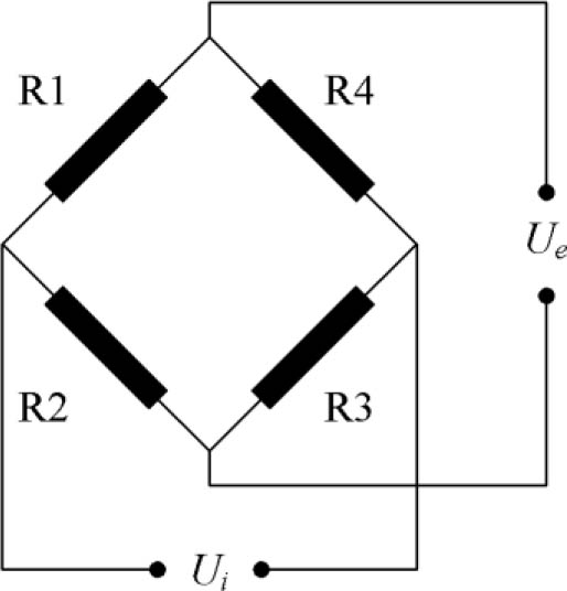
Fig. 1.
The Wheatstone bridge.
Finally, the VC matrix of the balance is established by representing the balance bridge outputs as polynomial functions of the component loads.
3. Case study
This section presents a case study to evaluate the feasibility of the VC method. A VC matrix established from the FEA model of a six-component strain gauge balance (hereafter referred to as the investigated balance) is compared with the SC matrix of the same balance. The balance (see Fig. 2) is a rear sting strain gauge balance with a diameter of 86 mm, a length of 569 mm, and is constructed from a single piece of high-strength maraging steel. Its material properties include a yield strength of 1754 N/mm2, an elastic modulus of 187250 N/mm2, and a shear modulus of 72000 N/mm2. The design loads for the force and moment components of the investigated balance are listed in Table 1.
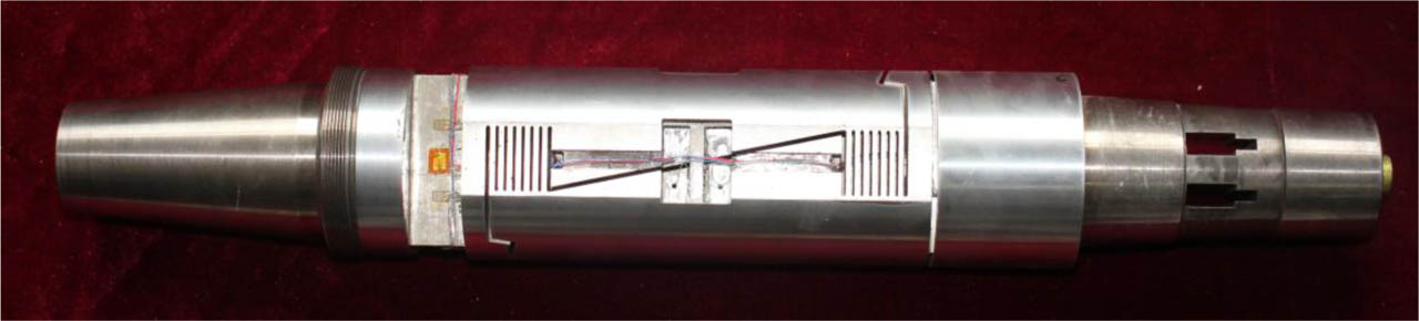
Fig. 2.
Photograph of the investigated balance.
Table 1.
Design loads for the investigated balance.
| Component | Fy [N] | Mz [N·m] | Fx [N] | Mx [N·m] | Fz [N] | My [N·m] |
|---|---|---|---|---|---|---|
| Design load | 18000 | 1800 | 1500 | 1200 | 4000 | 1200 |
A. Virtual calibration for balance
The VC of the investigated balance was performed using FEA software. To reduce computational cost, the FEA model for VC included only the balance element structure, excluding the calibration sting. The 3D model was imported into the FEA software to accurately determine the strain at the center of the strain gauge on the balance under applied loads. Hexahedral solid elements with a mesh control size of 1 mm were used for all measuring beams, while tetrahedral elements with a mesh control size of 2 mm were used for the complex structural regions of the balance, resulting in a total of 501490 elements and 1224890 nodes. Fig. 3 shows the finite element mesh of the balance.
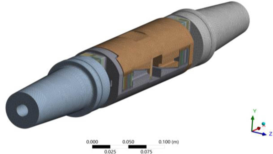
Fig. 3.
FEA mesh of the investigated balance.
The boundary conditions of the finite element model involve the balance’s fixed end, measuring end, and calibration center. To simulate the actual force state of body-axis calibration, a fixed constraint is applied to the measuring end during the virtual simulation, while loading conditions are applied to the fixed end. Specifically, force loads are applied to the fixed end via a remote force rigidly connected to the balance calibration center, and moment loads are applied directly to the fixed end. This inverted loading method effectively prevents parasitic load components in other directions that would otherwise be induced by elastic deformation of the measuring end in conventional setups, where the fixed end is constrained, and loads are applied at the measuring end.
The core of the virtual simulation calibration for the investigated balance lies in accurately simulating structural non-linear deformation. To achieve this, it is necessary to simulate the step-loading method for SC in each load case (with no fewer than 3 load steps per case) and activate the large deflection option in the solver settings. This approach effectively captures the structural stiffness variations induced by geometric non-linear deformation of the balance, thereby enabling precise determination of the non-linear term coefficients in the balance formula.
Assuming linear elastic behavior and material isotropy in the investigated balance, loading is applied only in the positive direction for each component during the VC. The strain analysis of the balance includes single-component loading and two-component loading. For a six-component balance, the simulation analysis includes 21 load steps.
The single-component loading includes:
The two-component loading includes:
Each loading case involves a 3-step sequence, with loads of 1/3Fi,design, 2/3Fi,design, and Fi,design respectively. These structured data points are subsequently utilized for the least-squares fitting.
After the above load steps are applied to the FEA model of the investigated balance, the solutions are computed sequentially. The strains are then extracted from the bonding positions of strain gauges on the balance, and the output of each bridge is obtained using (2). For comparison, the balance supply voltage Ue is set to 10 V, consistent with the value used in the actual SC. The nominal gauge factor of the strain gauge k is set to 2.25 for the Fy, Mz, Fx, Fz, and My components, and to 1.9 for the Mx component based on the gauge factor supplied with the gage packages. Using the bridge outputs and applied loads, the mathematical model coefficients are obtained via the least-squares method, from which the VC matrix for the balance is derived.
The bridge outputs of the investigated balance are defined as ΔUB1 to ΔUB6. Based on the measurement principle of the moment balance, ΔUB1 and ΔUB2 are used in combination for the Fy and Mz components; ΔUB3 and ΔUB4 are used for the Fx and Mx components, respectively; ΔUB5 and ΔUB6 are used in combination for the Fz and My components. The equations for the bridge outputs are as follows:
The VC matrix of the investigated balance (see Table 2) was calculated from the bridge outputs and applied loads.
Table 2.
The VC matrix of the investigated balance.
| Component | Fy | Mz | Fx | Mx | Fz | My |
|---|---|---|---|---|---|---|
| Csen | 12236.95 | 1379.64 | 3506.15 | 2638.97 | 5350.37 | 603.80 |
| Fy | 0 | 0.0004275 | 0.0222331 | −0.0001753 | −0.000006 | 0.0000006 |
| Mz | 0.0130928 | 0 | −0.0229588 | −0.0008566 | −0.0000507 | 0.0000066 |
| Fx | −0.0038566 | 0.0000002 | 0 | 0.0000015 | −0.0000023 | 0.0000003 |
| Mx | 0.0008202 | 0.0000622 | 0.001513 | 0 | −0.0002015 | 0.0043991 |
| Fz | 0.0000904 | 0.000006 | −0.000049 | −0.0007502 | 0 | 0.0000102 |
| My | −0.000352 | −0.0000829 | −0.0012826 | −0.1637126 | −0.0008886 | 0 |
| Fy*Fy | 0.00E+00 | 7.94E–10 | 9.00E–08 | −3.50E–11 | 1.46E–10 | 1.46E–12 |
| Mz*Mz | 1.21E–07 | 0.00E+00 | −6.20E–06 | −3.57E–09 | −1.14E–08 | −1.77E–09 |
| Fx*Fx | −5.31E–09 | −8.31E–10 | 0.00E+00 | −1.66E–11 | −3.10E–10 | −3.50E–11 |
| Mx*Mx | 4.91E–06 | −4.58E–07 | −2.80E–05 | 0.00E+00 | 4.36E–09 | 3.17E–10 |
| Fz*Fz | −8.43E–09 | −1.53E–10 | 1.56E–07 | 1.75E–10 | 0.00E+00 | 1.18E–10 |
| My*My | 1.71E–06 | −2.99E–07 | 3.35E–06 | 1.08E–09 | 8.23E–08 | 0.00E+00 |
| Fy*Mz | 6.96E–09 | 6.36E–09 | 1.27E–06 | −6.90E–10 | −1.27E–09 | 1.64E–10 |
| Fy*Fx | 1.64E–08 | −7.12E–09 | 8.65E–07 | 1.45E–09 | −3.23E–09 | −1.29E–11 |
| Fy*Mx | 3.81E–09 | −6.22E–10 | 2.41E–08 | −7.98E–08 | 1.96E–06 | 1.64E–07 |
| Fy*Fz | 6.26E–10 | −1.45E–10 | −8.48E–11 | −1.09E–08 | −3.21E–09 | −5.60E–10 |
| Fy*My | 1.06E–08 | −2.21E–09 | −3.97E–09 | 2.80E–07 | −1.97E–07 | −3.23E–08 |
| Mz*Fx | −1.27E–06 | 1.94E–07 | −1.82E–07 | 1.45E–08 | 1.40E–08 | 2.52E–09 |
| Mz*Mx | −7.10E–08 | 9.59E–09 | 4.58E–08 | −4.76E–07 | −1.33E–05 | −1.98E–06 |
| Mz*Fz | 6.26E–09 | −4.00E–10 | 3.85E–09 | 2.18E–07 | −1.43E–07 | −8.15E–09 |
| Mz*My | −6.54E–08 | 4.22E–09 | −1.98E–08 | 4.63E–06 | 6.34E–07 | −7.66E–09 |
| Fx*Mx | 8.29E–09 | −6.48E–10 | −3.25E–08 | −1.58E–08 | −1.89E–07 | −2.18E–08 |
| Fx*Fz | 1.51E–09 | 5.69E–11 | −4.87E–09 | 2.52E–09 | −7.28E–08 | 1.72E–08 |
| Fx*My | 1.10E–08 | 6.32E–11 | 8.57E–09 | 4.94E–09 | 2.06E–06 | 2.84E–07 |
| Mx*Fz | −1.98E–06 | −6.51E–08 | 2.35E–07 | −1.64E–09 | 8.28E–09 | 9.96E–10 |
| Mx*My | −4.26E–05 | 6.91E–06 | 3.20E–05 | 1.50E–06 | 2.04E–08 | 5.51E–09 |
| Fz*My | 3.13E–07 | −1.33E–08 | −2.05E–06 | 1.24E–06 | 4.60E–09 | 2.94E–09 |
B. Balance static calibration results
A body axis calibration system was used to calibrate the investigated balance with a second-order polynomial function. The system employs a manual weight loading method with manual resetting and adjustments to align the measuring end of the balance, thereby ensuring that the direction of the applied load coincides with the balance body axis. The excitation voltage for the investigated balance is 10 V, and the bridge output signals are transmitted to a host computer via a high-precision data acquisition system for further processing.
The SC encompasses loading cases in four body-axis directions: ±Y and ±Z. Both single-component and two-component loadings follow a 6-step incremental loading and unloading sequence, totaling 528 loading points. When solving the balance calibration matrix, the zero-offset effects introduced by the loading adapter are effectively eliminated by averaging the results from the positive and negative loading directions. Fig. 4 shows the SC setup for the investigated balance. Table 3 presents the SC matrix of the investigated balance.
Table 3.
The SC matrix of the investigated balance.
| Component | Fy | Mz | Fx | Mx | Fz | My |
|---|---|---|---|---|---|---|
| Csen | 11922.80 | 1347.85 | 3332.67 | 2568.62 | 5228.89 | 589.48 |
| Fy | 0 | 0.000039 | 0.023591 | −0.000442 | 0.00341 | −0.00033 |
| Mz | 0.012108 | 0 | −0.023699 | −0.001481 | 0.031882 | −0.00421 |
| Fx | −0.004616 | −0.000054 | 0 | −0.000142 | 0.00025 | −0.000064 |
| Mx | 0.013668 | 0.002606 | 0.003022 | 0 | −0.007704 | −0.003265 |
| Fz | 0.007823 | −0.001112 | −0.001461 | 0.000561 | 0 | 0.000723 |
| My | 0.046364 | −0.010228 | −0.003349 | −0.160641 | 0.022733 | 0 |
| Fy*Fy | 0.00E+00 | 1.48E–09 | 1.16E–07 | 0.00E+00 | 8.63E–09 | 0.00E+00 |
| Mz*Mz | 9.22E–07 | 0.00E+00 | −5.63E–06 | −9.33E–08 | 1.14E–07 | 3.07E–08 |
| Fx*Fx | −1.54E–07 | 8.53E–09 | 0.00E+00 | 0.00E+00 | −9.21E–08 | 6.00E–09 |
| Mx*Mx | −2.52E–06 | 9.03E–08 | −2.75E–05 | 0.00E+00 | 3.90E–07 | 8.96E–08 |
| Fz*Fz | −7.88E–08 | 6.68E–09 | 1.72E–07 | 5.66E–09 | 0.00E+00 | 3.24E–09 |
| My*My | 8.30E–07 | −1.21E–07 | 3.54E–06 | −1.63E–08 | −5.79E–07 | 0.00E+00 |
| Fy*Mz | 2.22E–07 | −2.51E–08 | 1.36E–06 | −5.72E–08 | 1.52E–07 | −1.47E–08 |
| Fy*Fx | −2.24E–07 | 2.53E–08 | 8.94E–07 | 3.04E–09 | −1.84E–08 | 2.22E–09 |
| Fy*Mx | −2.60E–08 | 2.84E–07 | −4.76E–08 | −2.67E–07 | 2.19E–06 | 2.64E–07 |
| Fy*Fz | 0.00E+00 | 0.00E+00 | 0.00E+00 | 0.00E+00 | 0.00E+00 | 0.00E+00 |
| Fy*My | 0.00E+00 | 0.00E+00 | 0.00E+00 | 0.00E+00 | 0.00E+00 | 0.00E+00 |
| Mz*Fx | −1.29E–07 | 2.35E–07 | −3.91E–07 | −4.01E–08 | 3.38E–07 | 6.01E–10 |
| Mz*Mx | 9.44E–07 | −2.05E–07 | 6.60E–07 | −1.23E–06 | −5.32E–06 | −6.91E–07 |
| Mz*Fz | 0.00E+00 | 0.00E+00 | 0.00E+00 | 0.00E+00 | 0.00E+00 | 0.00E+00 |
| Mz*My | 0.00E+00 | 0.00E+00 | 0.00E+00 | 0.00E+00 | 0.00E+00 | 0.00E+00 |
| Fx*Mx | 5.84E–07 | 5.66E–08 | −1.93E–07 | 1.25E–07 | 8.95E–07 | −2.51E–07 |
| Fx*Fz | −8.84E–08 | −2.87E–09 | −3.11E–08 | −2.98E–08 | −1.08E–07 | −3.95E–08 |
| Fx*My | 7.48E–07 | 7.17E–08 | −4.62E–07 | 2.25E–07 | 1.35E–06 | 4.26E–07 |
| Mx*Fz | −6.13E–07 | 3.43E–07 | 1.62E–06 | −3.65E–07 | 3.36E–07 | 9.47E–08 |
| Mx*My | −3.00E–06 | 1.79E–07 | 3.14E–05 | −1.17E–07 | −2.56E–07 | −6.27E–07 |
| Fz*My | 3.37E–07 | −2.93E–08 | −2.17E–06 | 3.60E–08 | −1.09E–06 | −1.62E–07 |
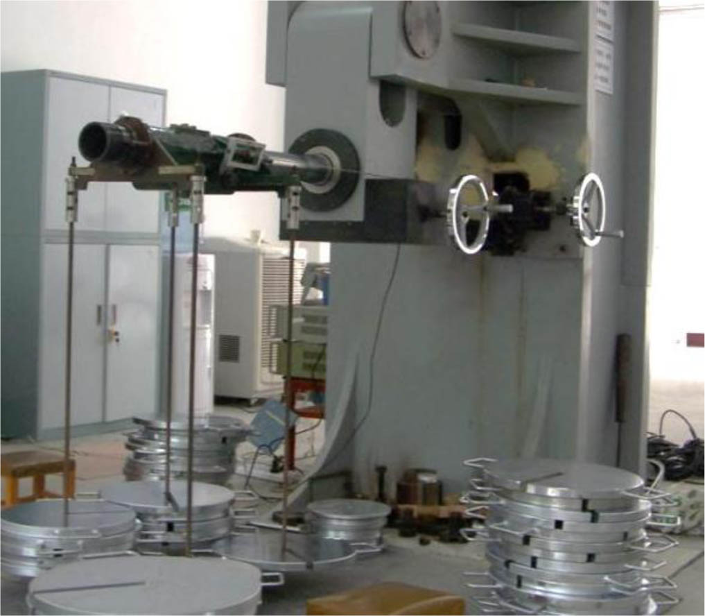
Fig. 4.
The SC setup for the investigated balance.
4. Results and discussion
To assess the consistency between the VC and SC matrices of the investigated balance, comparisons are presented for the sensitivity coefficients and the percent interaction of first-order linear terms, second-order terms, and cross-product terms. Here, the percent interaction is defined as the ratio of the interaction load derived from the interaction terms of the calibration matrix to the corresponding design load.
Table 4 compares the sensitivity coefficients of the VC and SC matrices. For the Fy, Mz, Fz, My, and Mx components, the relative errors of the sensitivity coefficients with respect to the SC range from 2.3 % to 2.7 %; for the Fx component, the relative error is 5.2 %.
Table 4.
Comparison of sensitivity coefficients.
| Component | Fy | Mz | Fx | Mx | Fz | My |
|---|---|---|---|---|---|---|
| VC [N/(mV/V) or N·m/(mV/V)] | 12236.95 | 1379.64 | 3506.15 | 2638.97 | 5350.37 | 603.80 |
| SC [N/(mV/V) or N·m/(mV/V)] | 11922.80 | 1347.85 | 3332.67 | 2568.62 | 5228.89 | 589.48 |
| Relative error [%] | 2.6 | 2.4 | 5.2 | 2.7 | 2.3 | 2.4 |
The discrepancies in sensitivity coefficients primarily stem from the strain gauge bonding positions, in addition to the dispersion of the balance material's mechanical properties [20] (which can exceed 2 % according to engineering experience), and the nominal gauge factor tolerance of the strain gauges (which can range from 0.5 % to 1 % as supplied by the gage packages). The strain gauge bonding positions have a significant effect on the bridge outputs of the balance, particularly for the Fy, Fz, Fx, and Mx components. Since the outputs are proportional to the strain, the measured strain ε of each component can be used to evaluate the uncertainty of the corresponding sensitivity coefficient. For the Fy, Fz, and Fx components, the strain as a function of length is given by the following equation:
where ε(L±ΔL) is the strain at the actual bonding position (L±ΔL) under load, εnor is the strain at the ideal position L under load, and ΔL is the position tolerance.In this case, the strain gauge bonding position for Fy and Fz components is 112.5 ± 0.5 mm (see Fig. 5), which leads to a maximum deviation of 0.44 % in the sensitivity coefficient; the bonding position for the Fx component is 15 ± 0.5 mm (see Fig. 5), which leads to a maximum deviation of 3.3 % in the sensitivity coefficient.

Fig. 5.
The schematic diagram of the strain gauge bonding position on the investigated balance.
For the Mx component, the strain gauge axes are inclined at 45° to the longitudinal axis of the investigated balance. The strain as a function of the angular misalignment is given by:
where ε(45±Δθ) is the strain at the actual bonding position under load; εX is the normal strain along the X-axis; εY is the normal strain along the Y-axis; γnor is the shear strain in the XY plane; and Δθ is the angular misalignment between the actual and ideal positions.The strain gauge bonding position for the Mx component is 45° ± 1° (see Fig. 5), resulting in a maximum deviation of 0.06% in the sensitivity coefficient.
Based on the above analysis, the VC results are considered reasonable.
Table 5 compares the percent interactions of the first-order linear terms between the VC and SC matrices. Fig. 6 shows the linear interactions of other components on the Fx component. The differences in interactions between the two calibration methods range from –3.47 % to 1.67 %, which are relatively small. It is noted that the first-order linear term interactions of the Fz and My components in the SC are slightly larger than those in the VC, at 3.43 % and –1.22 %, respectively. The main reason for this discrepancy is that the balance calibration roll angle cannot be maintained strictly level, whereas the VC is performed under ideal conditions.
Table 5.
Comparison of first-order linear terms between the VC and SC matrices.
| Component | Fy | Mz | Fx | Mx | Fz | My |
|---|---|---|---|---|---|---|
| VC [% FS] | 0.10 | 0.43 | 23.93 | −17.01 | −0.04 | 0.45 |
| SC [% FS] | 0.66 | −0.72 | 25.05 | −16.78 | 3.43 | −1.22 |
| Differences [% FS] | −0.56 | 1.15 | −1.12 | −0.23 | −3.47 | 1.67 |
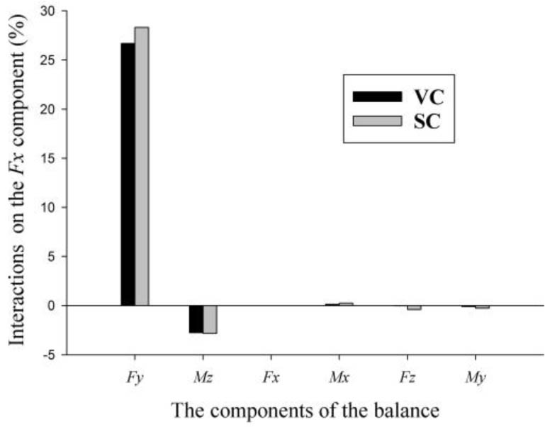
Fig. 6.
First-order linear interactions on the Fx component.
Table 6 compares the percent interactions of quadratic terms between the VC and SC matrices. Fig. 7 shows the quadratic term interactions of other components on the Fx component. The maximum difference of –0.75 % is observed with the Fx component.
Table 6.
Comparison of quadratic interactions.
| Component | Fy | Mz | Fx | Mx | Fz | My |
|---|---|---|---|---|---|---|
| VC [% FS] | 0.05 | −0.05 | −1.59 | 0.00 | 0.01 | 0.00 |
| SC [% FS] | −0.01 | 0.03 | −0.84 | −0.02 | 0.07 | 0.02 |
| Differences [% FS] | 0.06 | −0.08 | −0.75 | 0.02 | −0.06 | −0.02 |
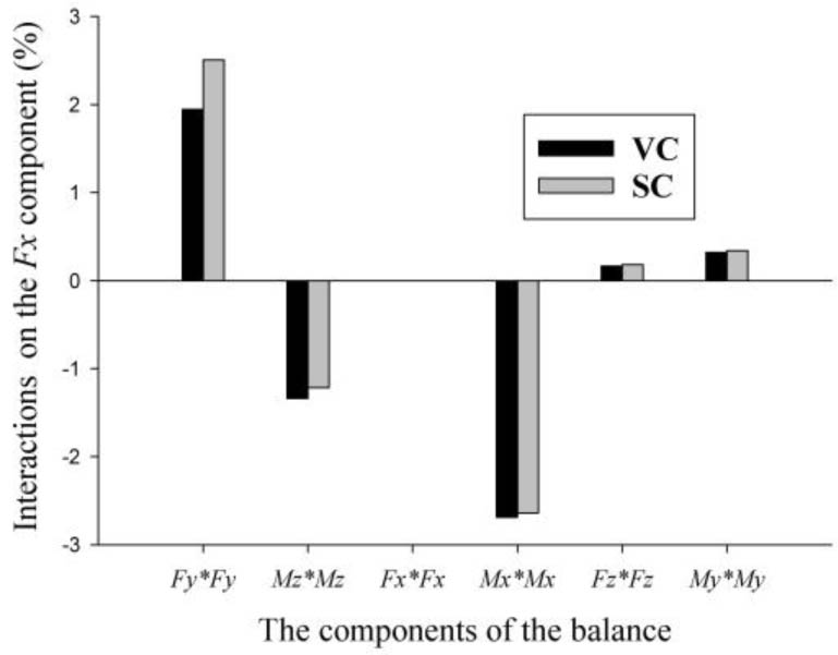
Fig. 7.
Quadratic interactions on the Fx component.
Table 7 compares the percent interactions of cross-product terms between the VC and SC matrices. The maximum difference between the two, 2.82 %, is observed for the Mx component. Fig. 8 shows the cross-product term interactions of other components on the Fx component between the VC and SC matrices, demonstrating relatively good agreement. The cross-product and quadratic term interactions in the calibration matrix are attributed to deformation of the balance under single or combined loads. In fact, according to FEA principles, the structural deformation results from FEA show good agreement with the actual deformation.
Table 7.
Comparison of interactions of cross-product terms.
| Component | Fy | Mz | Fx | Mx | Fz | My |
|---|---|---|---|---|---|---|
| VC [% FS] | −0.40 | 0.56 | 6.78 | 1.85 | 0.31 | −0.08 |
| SC [% FS] | −0.01 | 0.45 | 7.25 | −0.97 | 1.02 | 0.22 |
| Differences [% FS] | −0.39 | 0.11 | −0.47 | 2.82 | −0.71 | −0.3 |
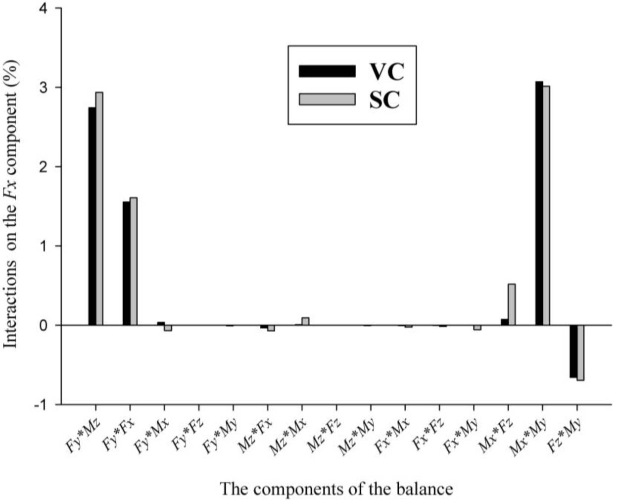
Fig. 8.
Cross-product term interactions on the Fx component.
Finally, Table 8 provides a comprehensive comparison of the percent interactions across all interaction terms between the VC and SC matrices. The overall differences in percent interactions between the two calibration methods range from –4.23 % to 2.61 %, further confirming that the VC matrix is in good agreement with the actual SC matrix.
5. Conclusions
This paper presents a VC method for strain gauge balances based on non-linear FEA. The sensitivity coefficients, first-order linear terms, second-order terms, cross-product terms, and all interaction terms of the VC matrix show relatively good agreement with those of the actual SC matrix for the investigated balance.
Consequently, the VC method can accurately predict the SC matrix of a six-component balance at its development stage and yield more reliable design results during balance development. This method improves the design quality and first-attempt success rate of balance development, thereby reducing overall costs and enhancing research and development efficiency.
Acknowledgements
The authors thank Fan Zhang for completing the static calibration of the investigated balance.