
1. Introduction
Train speed and position estimation are fundamental to safe railway operation. Accurate determination of these parameters is essential for both train drivers and railway operators [1]. Modern railway positioning systems use a hybrid architecture that combines onboard equipment with wayside facilities. Onboard equipment includes sensors and electronic units, whereas wayside facilities comprise fixed ground tags (balises) and track circuits. Balises provide absolute position references, while track circuits enable continuous monitoring of train occupancy. Satellite positioning technologies can also complement these systems [2], [3], [4]. Reliable speed and position estimation is critical for maintaining safe braking distances and optimising traffic management.
Odometry is an onboard system used to estimate train speed and travelled distance. Errors in position estimation can lead to unsafe distance calculations and impair braking performance. Modern systems, such as the European Train Control System, use multiple sensors simultaneously to obtain reliable speed estimates. However, none of these sensors is free from limitations. Environmental conditions can change unpredictably during operation, introducing additional sources of speed error [5].
A. Speed measurement technologies
Wheel-and-axle speed sensors (tachometers) are widely used because they are cost-effective and practical. They operate on various principles, including optical, Hall effect, variable reluctance, magnetic marker, current injection, and eddy current sensing [6]. These sensors convert wheel rotational speed into an electrical pulse frequency. However, they are highly sensitive to wheel slip and slide, particularly during acceleration and braking [5], [4], [7]. Their accuracy also depends on wheel diameter, which gradually decreases due to wear [7].
Doppler radar determines velocity from the Doppler shift of reflected signals. Measurement errors may arise from longitudinal vibrations and inaccuracies in the installation angle [4]. Under adverse weather conditions, such as water splashes, multipath propagation and ghosting effects may occur [7]. Performance deteriorates further in winter because accumulated snow can impair wave propagation, reducing the strength of reflected signals and degrading sensor performance.
Inertial Measurement Units (IMUs) utilise triaxial accelerometers and gyroscopes. Modern sensors are typically compact micro-electro-mechanical systems devices, characterised by low cost and relatively high noise levels [4]. Major error sources include sensor noise, scale-factor deviations, cross-axis coupling, and bias. IMU outputs are processed using inertial navigation system (INS) algorithms to estimate position, velocity, and attitude [4]. Accuracy degrades over time because integration errors accumulate and noise-induced drift increases during prolonged operation [8], [3].
Global Navigation Satellite Systems (GNSS), such as the United States Global Positioning System (GPS), are widely used in automotive applications and can also be utilised in railway systems. Signal reception is unavailable in tunnels, dense vegetation, and urban canyons [8], [1]. GNSS measurements are affected by noise. Position accuracy can be improved through map-matching, which identifies the closest point on the track [3]. Limited GNSS availability remains one of the main reasons for integrating supplementary sensors [1].
Eddy current sensors are another technology used for railway speed measurement [1]. The system consists of two sensors and a correlator. The sensors detect rail irregularities and generate two similar signals separated by a transit time corresponding to train speed [9]. Performance is largely unaffected by adverse weather conditions. They can also identify turnouts, which serve as natural beacons for position referencing [10]. However, the low installation height (approximately 10 cm above the rail head) and sensitivity to vertical motion hinder wider adoption.
Vision-based methods estimate train speed using at least two cameras that track distinctive points. Roadside feature recognition performs well under adequate illumination. It fails in low light, adverse weather, or when the optical path is obscured by dirt or dust [7], [2]. Light Detection and Ranging (LiDAR) systems with point-cloud matching overcome the illumination limitations of optical imaging. However, their resolution depends on visibility and deteriorates in severe weather conditions. Laser ranging systems have low architectural complexity but suffer from position divergence in feature-sparse environments [2].
Other methods exist, such as traction motor current measurements, but they also have inherent limitations [5], [11], [12]. Mobile communication-based positioning solutions can utilise existing infrastructure. However, they exhibit significantly larger positioning errors in environments with strong multipath effects, such as tunnels [2].
B. Fusion methods for train speed estimation
When multiple information sources are available, a fusion method becomes essential. The most widely used approach is based on variants of the Kalman Filter (KF) [8]. For train speed estimation and positioning, embedded multi-sensor technology compensates for wheel wear, idler diameter changes, and sliding during operation. It may employ the Federated KF algorithm for robust information processing [4]. Stochastic filters, such as the Extended KF (EKF), improve INS performance by reducing integration errors [5].
Fusion of IMU and tachometric signals has been implemented using two KFs and advanced procedures. These include adaptive matrix tuning and experimentally derived thresholds [5]. Railway odometry algorithms have also been validated using Hardware-in-the-Loop (HIL) simulators. For example, odometry developments related to the Italian SCMT system were evaluated with a dedicated dynamic simulator. The simulator was based on an industrial robot that reproduced railway vehicle motion and provided realistic inputs to inertial sensors and localisation algorithms. Such test platforms enable repeatable assessment of odometry performance under degraded adhesion and other critical operating conditions before on-track deployment [5]. This level of complexity makes tuning and maintenance more challenging.
Highly complex algorithms and multi-source fusion introduce significant computational demands and may prevent timely calculations [2]. KF has also been applied to fuse IMU, GNSS, tachometer, and map data [3].
KF was developed for linear systems and assumes Gaussian white noise, which makes it unsuitable for nonlinear train positioning. The EKF is widely used for nonlinear problems but neglects higher-order terms. The Invariant Extended KF improves convergence and observability-related stability and has been successfully applied in navigation and visual-inertial odometry. The process noise covariance matrix and the measurement noise covariance matrix are critical for filter performance. The Adaptive Extended KF dynamically adjusts noise parameters [8]. Fusion methods for train positioning and speed estimation also have drawbacks, including limited adaptability, high engineering costs, maintenance effort, and complex operating conditions [4]. In addition, they rely solely on noise models and do not account for systematic effects. This article considers systematic errors during the fusion process.
Artificial intelligence-based methods have also been proposed for railway applications. They can predict position information when GNSS signals are unavailable. However, these methods face challenges related to model complexity and computational efficiency. Balancing accuracy and efficiency remains essential in odometry applications [8]. Moving computations to cloud platforms introduces unpredictable communication latency, which is unacceptable for braking control. Edge computing enables rapid sensing and processing of large volumes of sensor data to support decision-making, but it also faces limitations under dynamic conditions. This approach assumes onboard sensors and a ground-based edge server connected through wireless communication. Reliable communication across an entire railway network in all weather conditions is extremely difficult to guarantee [2].
The limitations of existing solutions motivate the approach adopted in this work, which does not require high computational power. Train speed is estimated using weighted signals from multiple sensors. The weights are determined from both random components, such as noise, and systematic components. Estimation errors are calculated using the reference speed assumed in the simulations. The resulting estimates are compared with means and medians, which are among the simplest statistical measures available. This study extends previous work [13] and provides a detailed description of the weight calculation method. In addition, one sensor is intentionally made to deviate significantly from the reference value to assess the robustness of the estimates.
2. Subject & Methods
A hypothetical train speed profile is analysed. The train passes a balise at the 100 m mark whilst travelling at 100 km/h. The driver then applies the brakes, following the deceleration profile shown in Fig. 1 (green curve). The deceleration increases linearly and reaches 55 cm/s2 after 2.75 s. When the vehicle speed falls below 10 km/h, the deceleration gradually decreases until the train comes to a standstill. As a result, the train speed decreases as shown by the blue curve. This speed profile serves as the reference for the subsequent analysis.
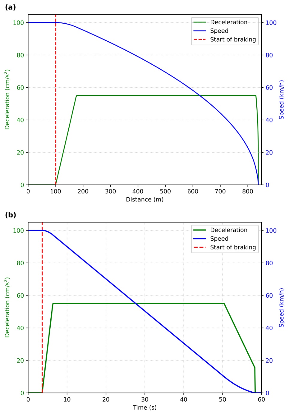
Fig. 1.
Reference deceleration and speed profiles utilised for simulation analysis in function of distance (a) and time (b).
This work considers five sensors: an accelerometer, two wheel speed sensors (WS1 and WS2), a Doppler radar, and a GPS. Sensor speed offsets are assumed to be reset at the balise, unlike in practice, where only distance offsets are reset. Sensor measurements are updated every h = 100 ms. For each sensor and each sample, the instantaneous speed is calculated. Random and systematic error components are then estimated for each sensor.
Maximum permissible errors follow the relevant technical notes. In the simulations, the applied error magnitudes are set to approximately 70–80 % of these limits. Further details are provided below.
Where required, random errors are combined using the root-sum-of-squares method. Systematic errors are combined using a worst-case approach by summing absolute contributions [14]. The standard uncertainty, u, is calculated in accordance with [15]:
Here, σ denotes the estimated standard deviation of the random error. The term Δmax denotes the maximum systematic error. In the simulations, the noise standard deviation added to the reference value is set slightly lower. Likewise, the offsets applied in the simulations are smaller than the maximum systematic error.
For all sensors, measurement errors are represented by random and systematic components. The random component of quantity X is denoted by ΔrX, whereas the systematic component is denoted by ΔsX. Random contributions are combined using the root-sum-of-squares method, while systematic contributions are combined using a worst-case approach. The resulting combined standard uncertainty is denoted by u(X).
A. Accelerometer
It measures longitudinal deceleration, which is integrated to obtain speed. The measured deceleration, aAcc, is modelled as
where aref denotes the reference deceleration. This follows the deceleration profile shown in Fig. 1. The parameter GAcc represents the relative gain error.The noise term εAcc is modelled as a Gaussian random variable:
Here, a0Acc is the accelerometer bias, which causes drift in the integrated speed estimate. The noise standard deviation is σAcc. For uncertainty evaluation, the following values are used:
For the simulation study, the following values are used:
The speed provided by the accelerometer for the ith sample is calculated from the measured deceleration using Euler integration:
In the next step, the speed uncertainty is assessed. The random component, ΔraAcc,i, is characterised by σAcc. The systematic component (maximum error) is calculated as
The combined uncertainty of deceleration is calculated as
assuming a uniform distribution for the systematic component.
The simulation results are shown in Fig. 2. The permissible error bands in Fig. 2(b) and (c), corresponding to ±2u(aAcc,i), are calculated using (6). They are expected to contain 95 % of the reference values.
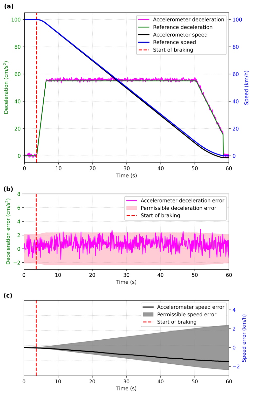
Fig. 2.
Accelerometer-derived deceleration and speed compared with the reference profiles (a). Deceleration errors (b) and speed errors (c) with respect to the corresponding permissible error bands.
Propagation of random errors is based on the root-sum-of-squares method. The error sources are assumed to be independent, and the individual contributions follow from (4):
The jitter of the sampling interval is assumed to be Δrh = 1 ms.
The systematic component is propagated using a worst-case sum of absolute contributions:
Because Δsh = 0 is assumed, the term |aAcc,i · Δsh| is omitted.
The combined uncertainty of speed is calculated as
A uniform distribution is assumed for the systematic component.
The resulting speed estimate is shown in black in Fig. 2(a). Due to the accumulation of systematic errors in this sensor, a non-zero speed remains at standstill.
B. Wheel sensors WS1 and WS2
They measure axle rotations; therefore, their output signal vWSn is proportional to the vehicle speed:
where n = 1, 2 denotes the sensor index. The systematic gain error results from changes in wheel diameter during operation. Here, NDn denotes the nominal diameter of WSn, and ADn denotes the actual diameter. The parameter σWSn represents sensor noise.Values used for uncertainty evaluation:
Values used in simulations:
Next, the speed uncertainty is evaluated. The random error component ΔrvWSn is characterised by σWSn. The systematic component, representing the maximum error, is derived from GWSn·vWSn.
The combined standard uncertainty of speed is:
assuming a uniform distribution for the systematic component.To simulate a wheel slide, the WS1 readings between 20 s and 21 s are set to zero. During this interval, u(vWS1) = 35 km/h. A more sophisticated uncertainty assessment could be used. However, this approach is sufficient to illustrate the operation of the algorithm.
C. Doppler radar
It measures signals reflected from trackside ballast, which are proportional to the vehicle speed:
Values used for uncertainty evaluation:
Values used in simulations:
The speed uncertainty is assessed similarly to the wheel sensors. The random component ΔrvRadar = σRadar, and the systematic component ΔsvRadar = v0Radar.
The combined standard uncertainty is:
D. GPS
It measures signals received from satellites. Its output is modelled as:
Values used for uncertainty evaluation:
Values used in simulations:
The random component is ΔrvGPS = σGPS, and the systematic component is ΔsvGPS = v0GPS. The combined standard uncertainty is:
assuming a uniform distribution for the systematic component.Fused values can be obtained using several approaches. The most common approach uses mean values and performs well when many sources have normally distributed errors. When only a few sensors are available, medians often provide more reliable estimates.
Another approach accounts for the uncertainties of the measured quantities. The weighted method estimates the fused value y from sensor values xi and their uncertainties ui as described in [16]:
In this work, only the estimation error relative to the reference speed known from the simulation is analysed. The uncertainty of the speed estimate obtained using the weighted method is not derived explicitly. Its evaluation would require separate treatment of the random and systematic components. The resulting expression would be lengthy and provide no additional insight into the problem considered in this article.
KF is another widely used fusion method that combines measurements from multiple sensors [17], [18]. However, its weighting mechanism is based on measurement noise covariance and therefore considers only random error components. In contrast, the method proposed in this work accounts for uncertainties that include both random and systematic effects.
3. Results and Discussion
Based on the assumed values and measurement models, speed profiles for all sensors, their uncertainties, and fused speeds obtained using three methods were calculated. The results are briefly discussed below.
Fig. 3 shows the expanded uncertainties of all sensors, calculated as twice their standard uncertainties. The accelerometer uncertainty increases over time due to its cumulative nature, despite being reset at the 100 m mark. The wheel sensor uncertainties decrease with speed during braking. WS1 shows a large uncertainty between 20 s and 21 s due to wheel slide. Radar and GPS have speed-independent uncertainties, with GPS exhibiting markedly poorer performance.
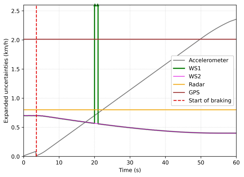
Fig. 3.
Expanded speed uncertainties of sensors as a function of time during deceleration.
Speeds measured by all analysed sensors are presented in Fig. 4. The measurements differ in both variability and permissible error bands. In the simulated experiment, the reference value (blue line) is known and can be compared directly with sensor outputs. In real-world experiments, the reference value can only be estimated using a fusion method.
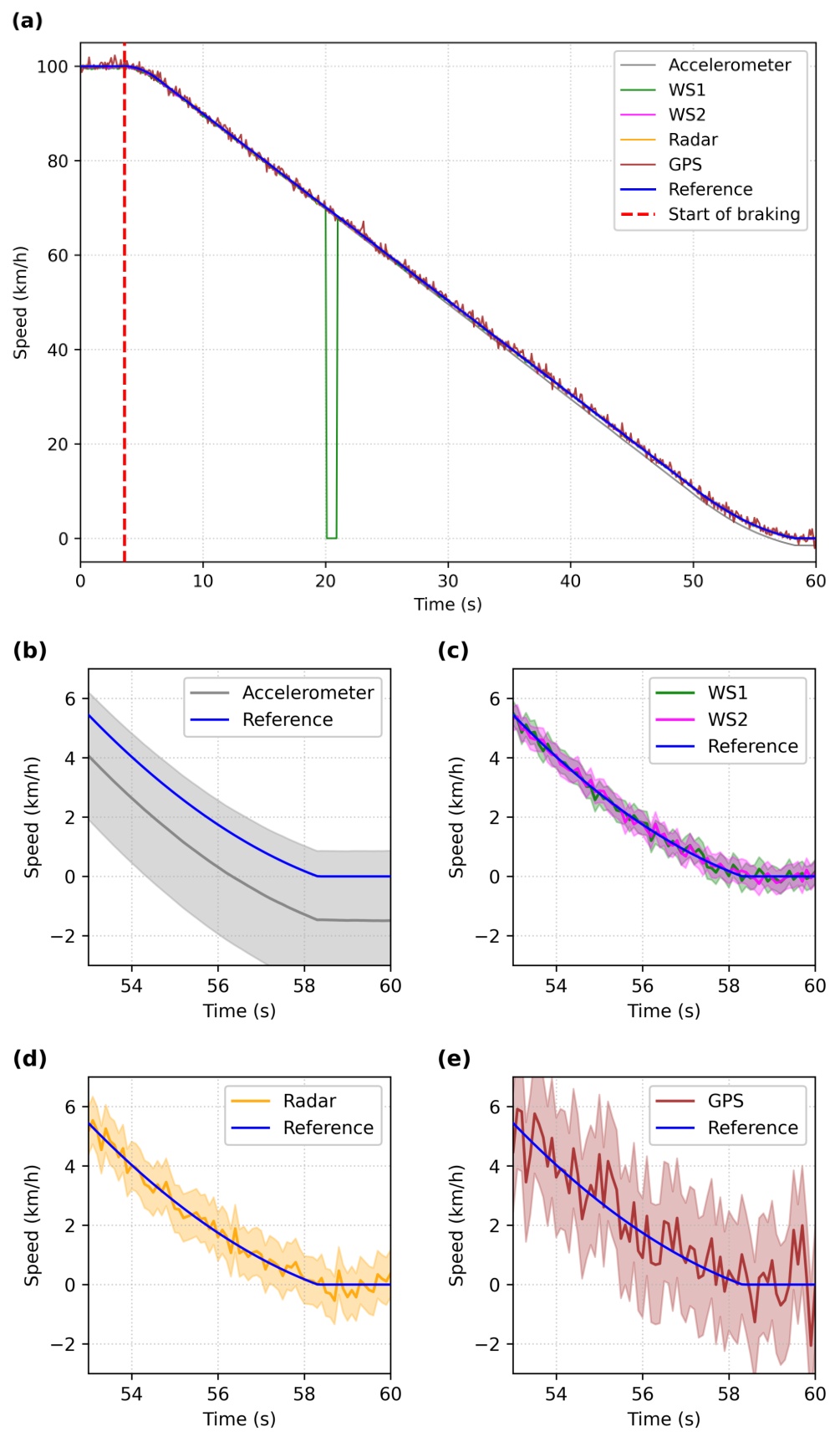
Fig. 4.
Sensor-measured speeds. Comparison of all measurements over the entire simulation period (a). Enlarged view of the last 7 seconds with permissible error bands for individual sensors (b–e).
Because the errors are much smaller than the measured speeds and therefore difficult to distinguish, they are shown separately in Fig. 5. The accelerometer exhibits a clear drift in speed error over time. WS1 shows errors below −2.5 km/h between 20 s and 21 s. Outside this interval, WS1 produces larger errors than WS2 because of differences in actual wheel diameter. GPS exhibits the widest spread of error values.
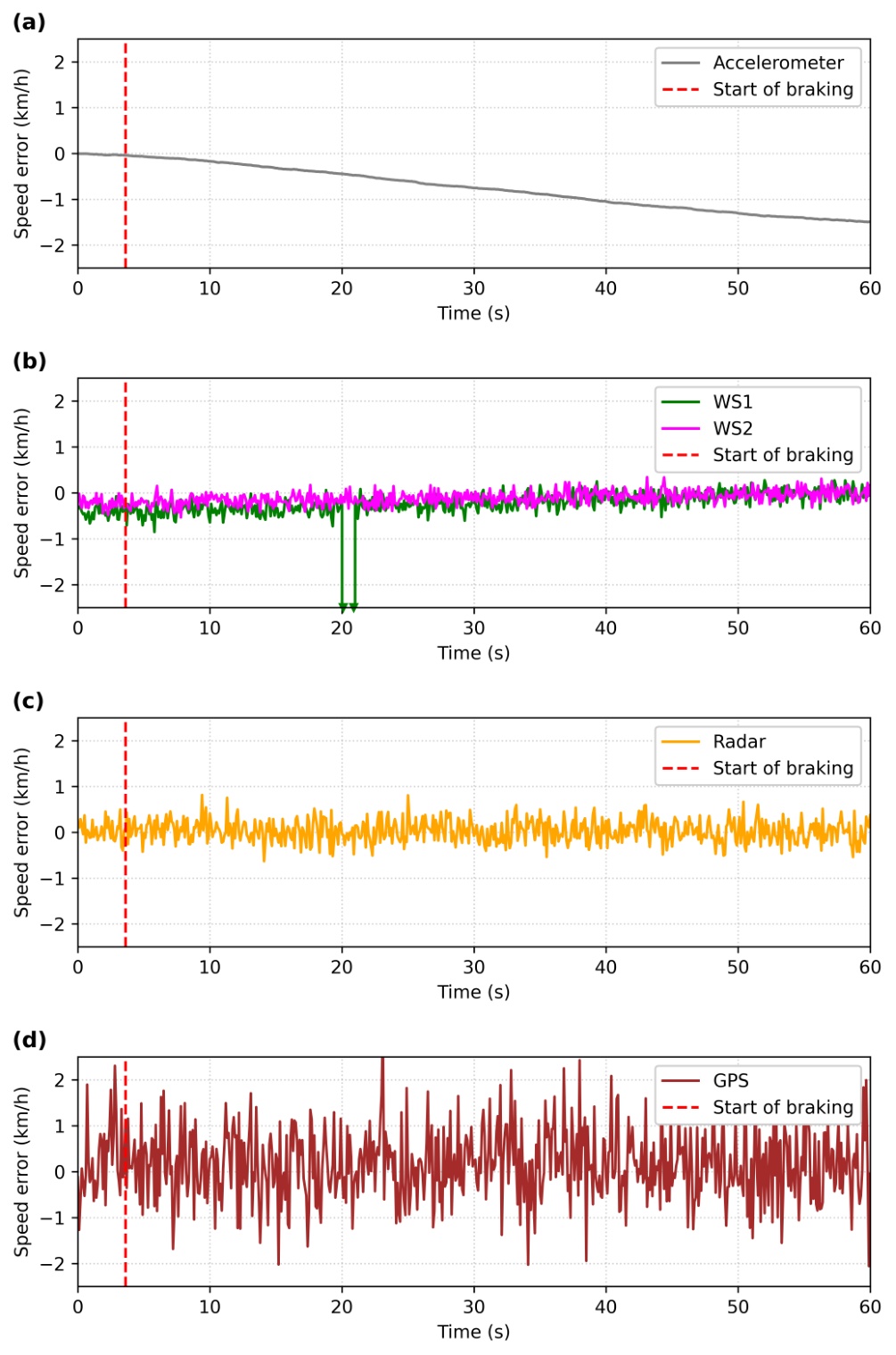
Fig. 5.
Comparison of sensor speed errors produced by the individual sensors.
Applying the fusion methods yields the results shown in Fig. 6. Panel (a), corresponding to the mean value, is the noisiest and shows the largest deviation from zero. During the wheel slide, the error becomes strongly negative and substantially reduces the estimated speed. The median values shown in panel (b) remain much closer to zero. During sliding, the errors stay within ±0.5 km/h, indicating a high degree of robustness to a single axle slide. Panel (c), corresponding to the weighted method, produces the smoothest estimate, particularly at the beginning when the accelerometer uncertainty is low.
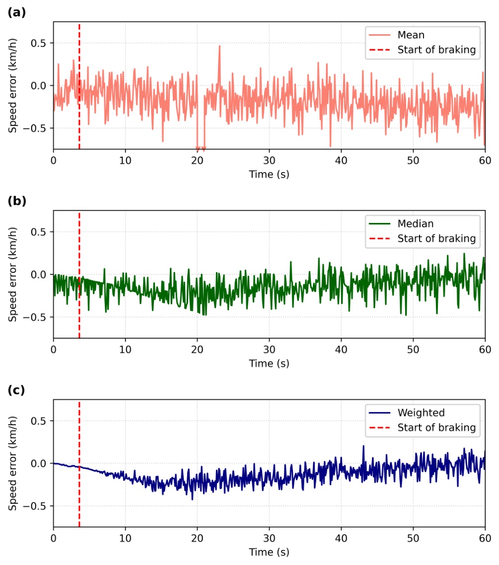
Fig. 6.
Fused speed error obtained using mean (a), median (b), and weighted (c) fusion methods.
The errors obtained with the weighted method are closest to zero. The standard deviations of the speed errors are 1.7, 0.14, and 0.11 km/h for the mean, median, and weighted methods, respectively. The values vary across simulations due to randomisation, but the weighted estimate consistently remains the most accurate. The order-of-magnitude increase in the mean reflects its high sensitivity to outliers caused by wheel slide.
4. Conclusions
This study investigates train speed estimation during a simulated braking manoeuvre. Five sensors were considered: an accelerometer, two wheel sensors, a Doppler radar, and a GPS. One wheel sensor experienced a one-second slide. Each sensor was described by a measurement model containing both systematic and random components. All error sources contributed to the measurement uncertainty. Random components were combined using the root-sum-square method, whereas systematic components were treated using the worst-case approach. The resulting standard uncertainties were used as weights during data fusion. The weighted estimates, together with the mean and median values, were compared against the reference speed. The results show that mean estimates are highly sensitive to wheel slide. Median-based estimates provide better accuracy. A slide on a single axle caused no noticeable change in the estimated speed. The most accurate results were obtained with the weighted method. However, this approach requires well-defined measurement models and engineering analysis of uncertainty contributions for each sensor.
Acknowledgment
This research was funded by the Polish Ministry of Science and Higher Education, under grant number 02/050/BK-26/0058.
The author used Copilot AI to improve the language and readability of the manuscript. The tool was used solely for linguistic editing and style refinement. All scientific content, analyses, interpretations, and conclusions were developed by the authors. No part of the manuscript content was generated by artificial intelligence.