
1. Introduction
As crucial supporting and transmission components in rotating machinery, the operating conditions of rolling bearings directly affect the reliability, safety, and maintenance costs of the equipment. Under the combined effects of long-term load, friction, impact, and complex environments, bearings are highly susceptible to faults such as wear, cracks, looseness, and misalignment. If these faults are not identified on time, they can lead to degraded equipment performance and unplanned downtime in mild cases, or trigger severe safety accidents in extreme cases. Therefore, bearing fault diagnosis under complex working conditions has always been a vital research direction in the field of machinery health monitoring. With advances in sensing technology, data acquisition techniques, and intelligent algorithms, data-driven diagnostic methods based on operational signals such as vibration, acoustics, and current have gradually become the mainstream, providing a new technical pathway for the condition recognition of complex mechanical systems [1], [2], [3].
In the research of vibration signal-driven fault diagnosis, feature extraction has always been a critical step that affects diagnostic performance. Early studies primarily focused on manual features in the time, frequency, and time-frequency domains. For instance, statistical indicators, impact metrics, harmonic components, and spectral features were extracted from vibration signals and combined with traditional classifiers like Support Vector Machines and K-Nearest Neighbors to achieve condition recognition. Cui et al. proposed a three-stage feature extraction and machine learning framework, analyzing data structures through unsupervised learning and screening key features via sensitivity analysis to mitigate overfitting under non-stationary conditions [1]. Daas et al. extracted statistical, harmonic, and spectral features from vibration signals and utilized ANOVA for feature selection to improve classification efficiency [4]. Subsequently, aiming at nonlinear, non-stationary, and heavily noisy vibration signals, researchers further introduced methods such as Variational Mode Decomposition, Complete Ensemble Empirical Mode Decomposition with Adaptive Noise, hierarchical decomposition, and envelope spectral entropy, enhancing weak fault information through a decomposition–reconstruction–feature construction approach. Yang et al. proposed a feature extraction method based on Variational Mode Decomposition (VMD) and improved envelope spectral entropy [5], while Chen et al. further introduced a hierarchically improved envelope spectral entropy method [6], both demonstrating the effectiveness of decomposition and entropy features in enhancing fault-sensitive information. In recent years, with the increasing demands of complex working conditions and multi-source perception, multi-domain, multi-channel, and multi-modal feature extraction have gradually gained significant attention. Cao et al. pointed out that multi-domain feature extraction outperforms single-domain feature extraction [7]. Luan et al. enhanced fault features under complex transmission paths through the weighted fusion of multi-channel vibration information [8]. Guan et al. utilized a time-frequency dual-branch structure to improve feature representation capabilities under different working conditions [9]. These studies indicate that a single representation is often insufficient to comprehensively describe complex fault mechanisms, and complementary multi-domain features have increasingly become a prominent trend in feature extraction research.
Regarding fault diagnosis models, research has transitioned from traditional machine learning to deep learning-driven automatic representation learning. Traditional diagnostic methods typically rely on manual features and shallow classifiers, whose performance is easily constrained by feature quality and prior experience. In contrast, deep models such as convolutional neural networks (CNN), temporal convolutional networks (TCN), bidirectional long short-term memory, ResNet, and Transformers can automatically learn fault-sensitive features in an end-to-end manner, thereby exhibiting stronger diagnostic capabilities in complex scenarios. For example, Liu et al. combined an improved spectral subtraction method with CNN–TCN in acoustic fault diagnosis, enhancing spatiotemporal feature modeling capabilities in highly noisy environments [10]. Luo et al. integrated CNN with BiLSTM, achieving high-precision recognition with multi-dimensional feature inputs [11]. Patil et al. employed a 1D-CNN to extract bearing defect and misalignment features automatically [12]. Concurrently, multi-modal and multi-branch structures have gradually become an important direction for improving diagnostic performance. Zaman et al. utilized a dual-input CNN to fuse acoustic emission and vibration signals [13], while Bi et al. improved diagnostic robustness under complex conditions through an acoustic–vibration dual-branch depthwise separable convolutional network [14]. Recently, diagnostic models based on Transformers and visual intelligence have also made significant progress. Khan et al. combined VMD, Continuous Wavelet Transform, and Vision Transformer to enhance global feature aggregation capability [15]. Zhang et al. proposed a trend-aware patch feature fusion Transformer to mine trend variation information in vibration signals [2]. Wang et al. enhanced fault image representation capabilities through multi-image feature extraction and attention fusion [16]. These studies indicate that current fault diagnosis models are evolving towards multi-branch, multi-modal, global modeling, and attention enhancement. Recent studies have further explored attention-enhanced deep networks and advanced vibration sensing strategies to improve feature representation and diagnostic robustness under complex operating conditions [25], [26].
Despite the significant progress in feature extraction and deep diagnostic models, variable working conditions in actual industrial scenarios still severely restrict the generalization application of these models. Due to the influence of factors such as load, rotational speed, environmental noise, installation methods, and individual equipment differences, the vibration data collected during the training and testing phases often exhibit significant distribution shifts. This causes models trained under the independent and identically distributed assumption to suffer a substantial performance drop under target working conditions. To address this issue, transfer learning and domain adaptation methods have been widely introduced into the fault diagnosis field. Their core idea is to learn domain-invariant features to reduce the distribution discrepancy between source and target domains, thereby improving the model’s diagnostic capability in the target domain. Han et al. proposed the Transfer Learning-based Multimodal Feature Fusion (TL-MMFF) model, dynamically weighting and fusing vibration time-frequency features and torque time-domain features, and combined it with Maximum Mean Discrepancy constraints to reduce the distribution difference of fused features under different conditions [3]. Yang et al. constructed a variable-condition fault diagnosis model based on Multiple Kernel Principal Component Analysis and domain-adaptive deep belief networks, utilizing Multiple Kernel Maximum Mean Discrepancy (MK-MMD) to enhance cross-domain generalization ability [17]. With the development of transfer learning, researchers have begun to further focus on multi-modal transfer and fine-grained domain alignment. Zhang et al. proposed the Multimodal Fault Diagnosis (MoMD) Transformer, transferring fault knowledge from the vibration modality to the current modality via knowledge transfer in scenarios with inconsistent modality availability [18]. Geng et al. proposed MCL-3WDA to achieve fine-grained domain alignment from the channel, layer, and category levels [19]. Zhang et al. combined physical priors, simulation pre-training, and category-level alignment through failure-mechanism-driven multi-adversarial domain transfer learning to mitigate the simulation-to-reality gap and negative transfer problems [20]. Furthermore, Su et al. combined meta-learning with multi-kernel MMD to enhance the model’s rapid adaptation capability to unknown conditions and small-sample target domains [21]. These works demonstrate that transfer learning has become a key technology in variable-condition fault diagnosis, evolving from global coarse-grained alignment to comprehensive frameworks that integrate multi-modality, fine-grained alignment, physical priors, and rapid adaptation mechanisms.
The remaining gap can be condensed into three coupled deficiencies. First, many cross-condition methods use a single representation, or concatenate heterogeneous inputs before their representation-specific structures have been fully extracted [22], [23], [24]; this weakens the complementarity between transient time–frequency textures and global harmonic distributions. Second, fixed concatenation or summation assigns the same importance to each representation for every sample, even though the reliability of Short-Time Fourier Transform (STFT) and Fast Fourier Transform (FFT) evidence varies with fault type and load. Third, aligning heterogeneous branches directly in their native spaces can mix representation discrepancy with operating-condition discrepancy. More elaborate alternatives frequently require target pseudo-labels, adversarial optimization, or additional sensing modalities, which introduces error propagation or training instability. Thus, the essential need is a compact framework that preserves representation-specific processing, performs sample-wise fusion, and aligns a well-defined common latent space.
The proposed framework differs from these approaches in four specific respects. Both views are generated from the same four-channel vibration segment, so the method does not require additional sensors or modalities. STFT and FFT are processed by heterogeneous CNN and TCN encoders chosen for their respective two-dimensional local-texture and one-dimensional long-range spectral structures. Their projected features are combined by a sample-adaptive softmax gate rather than by fixed fusion. Finally, normalized MK-MMD is applied only to the fused representation; no target labels, pseudo-labels, or adversarial discriminators are used. The main contributions are therefore summarized as follows:
(i) A same-segment dual-representation pipeline is proposed to retain complementary local time–frequency and global spectral evidence without introducing an extra sensing modality.
(ii) A heterogeneous CNN–TCN encoder with sample-adaptive gated fusion is designed to preserve representation-specific feature extraction before learning a common decision representation.
(iii) A fused-space MK-MMD objective is used for stable unsupervised cross-load alignment, and the framework is evaluated on all three many-to-one transfer directions with explicit sample counts, contemporary external baselines, A1–A5 ablations, and class-level analyses.
2. Subject & Methods
A. Signal representation and backbone modules
Vibration signals typically exhibit significant non-stationarity and time-varying characteristics. Relying solely on pure time-domain or pure frequency-domain analysis makes it difficult to simultaneously characterize the temporal location and frequency distribution of fault impulses. By introducing a sliding window function, the STFT partitions the original signal into a series of locally stationary segments and performs the Fourier transform within each local window, thereby achieving a joint representation of the signal in both the time and frequency domains. For a single-channel vibration signal x(t), its STFT can be expressed as
where w(t − τ) is the window function centered at τ, and f is the frequency variable. By calculating the magnitude of the complex spectrum and applying a logarithmic transformation, a stable time-frequency magnitude representation can be obtained asThe primary advantage of STFT lies in its ability to explicitly preserve the local time-frequency texture of fault signals, making it particularly effective for characterizing impulsive, modulating, and energy-mutational fault patterns. Therefore, STFT is used to map multi-channel vibration signals into multi-channel time-frequency spectrograms, which serve as the input representation for the spectral branch.
CNNs possess excellent local feature extraction capabilities in image recognition and pattern analysis. Their core idea is to share parameters via convolutional kernels within local receptive fields, extracting edges, textures, local structures, and high-level semantic features from the input data layer by layer. For mechanical fault diagnosis tasks, the time-frequency spectrograms obtained through STFT are essentially two-dimensional structured representations, where local frequency-band textures, impulse energy distributions, and neighborhood time-frequency correlations are all highly suitable for CNN modeling. The general form of a convolutional layer can be written as
where X and Y denote the input and output feature maps, respectively, W represents the convolutional kernel parameters, b is the bias term, and σ(·) denotes the nonlinear activation function.Temporal Convolutional Network is a class of convolutional neural network structures oriented towards sequence modeling tasks. Its core idea is to introduce causal convolutions, dilated convolutions, and residual connections based on one-dimensional convolutions, thereby effectively expanding the receptive field and enhancing the ability to model long-range dependencies while maintaining low parameter complexity. Compared with recurrent structures, TCNs offer advantages such as parallel computing efficiency, short gradient propagation paths, and more stable training. Therefore, it is adopted to model the FFT-based spectral sequence.
In addition, domain alignment is achieved through MK-MMD. Let the source-domain and target-domain feature distributions be denoted as 𝒟s and 𝒟t. The MK-MMD metric measures the discrepancy between them in a reproducing kernel Hilbert space induced by a set of kernels:
where and denote source-domain and target-domain features, respectively, ϕ(·) is the nonlinear mapping, and ℋk is the reproducing kernel Hilbert space induced by the multi-kernel function.B. Proposed dual-branch MK-MMD framework
Aiming at the issues of insufficient representation and domain distribution shift in rolling bearing fault signals under variable working conditions, a cross-domain fault diagnosis framework based on dual-domain complementary representation, heterogeneous dual-branch encoding, and MK-MMD domain alignment is proposed. Taking multi-channel vibration segments as input, the framework first constructs two complementary representations (see Fig. 1): the STFT time-frequency spectrogram representation, which preserves local non-stationary fault textures, and the FFT spectral sequence representation, which characterizes the global frequency-domain energy distribution. These two representations are then fed into a two-dimensional convolutional branch and a temporal convolutional branch, respectively, for feature extraction. Adaptive weighted integration of the dual-branch features is achieved through a gated fusion module. Finally, a classification objective and an MK-MMD domain alignment objective are introduced at the fused feature layer, thereby simultaneously guaranteeing the separability of fault categories and the consistency of cross-condition distributions.
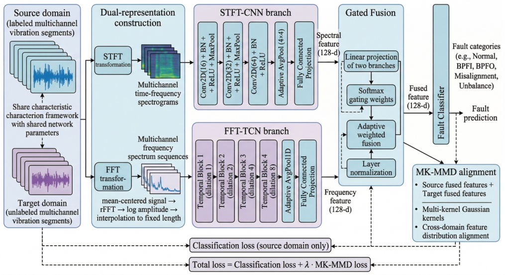
Fig. 1.
Overall structure of the proposed dual-branch fault diagnosis framework.
For the input multi-channel vibration samples, standardization is first applied to each channel to reduce amplitude scale differences across different channels. Subsequently, STFT is applied to each channel individually to obtain the corresponding local time-frequency complex spectrum, and the logarithmic magnitude is calculated to generate a two-dimensional time-frequency spectrogram. Let the signal of the c-th channel be denoted as x(c)(t); its time-frequency representation can be written as
The time-frequency spectrograms of all channels are stacked along the channel dimension to form a multi-channel spectrogram tensor, which is further globally normalized to serve as input to the spectral branch.
To compensate for the deficiency of the single STFT representation in modeling global spectral distribution, an FFT-based frequency-domain representation is further constructed. Mean removal is first performed on each channel signal to attenuate interference from the DC component. Subsequently, a real-valued FFT is applied to the mean-removed vibration sequence to obtain the one-sided spectrum. The logarithmic magnitude is then calculated to derive a stable frequency-domain representation:
Considering potential variations in spectral lengths across different samples, the spectra of all channels are uniformly resampled to a fixed length and stacked along the channel dimension to form a multi-channel spectral sequence tensor.
The STFT branch employs a two-dimensional convolutional structure to extract local discriminative features from multi-channel time-frequency spectrograms. Let the input spectrogram be denoted as S; the spectral-domain feature output by this branch is denoted as
where Es(·) represents the spectral-domain encoder. The FFT branch uses a TCN-based frequency-domain encoder to exploit long-range dependencies in the spectral sequence. Let the input spectral sequence be denoted as F; the feature output by the frequency-domain branch is where Ef(·) represents the TCN-based frequency-domain encoder.Since the STFT and FFT branches focus on local time-frequency textures and global frequency-domain structures, respectively, relying solely on features from a single branch makes it difficult to comprehensively characterize complex fault patterns. To address this, a gated fusion module is introduced to adaptively integrate the dual-branch features. Let fs and ff denote the spectral-domain and frequency-domain features, respectively. First, both are mapped into a unified fusion space:
Subsequently, a gating network is employed to generate the weight coefficients of the two branches:
The final fused feature can be expressed as
For labeled source-domain samples, cross-entropy loss is adopted for fault classification supervision. Let the true label of a source-domain sample be , and the predicted probability be . The classification loss is defined as
Integrating the classification objective and domain alignment objective, the total loss can be written as
where λ is the weight coefficient for domain alignment. To prevent excessive domain alignment from suppressing classifier learning in the early stages of training, a progressively increasing weight strategy is employed so that λ gradually rises from a small value to a preset maximum value during the initial epochs. In this study, the maximum alignment coefficient was set to λ = 0.25, determined through preliminary experiments on the source-validation set. And then fixed for all transfer tasks and final evaluations. No target-domain labels were involved in this selection process.C. Dataset, preprocessing, and experimental protocol
The experiments use the variable-load subset of the public KAIST rotating-machinery dataset reported by Jung et al. [27]. Only vibration measurements are used. Four accelerometer channels were recorded on the two bearing housings in orthogonal directions at 25.6 kHz and approximately 3010 rpm. The five labels are bearing inner-race fault (BPFI), bearing outer-race fault (BPFO), shaft misalignment, normal state, and rotor unbalance. Table 1 summarizes the measurement and preprocessing settings.
Table 1.
Measurement data and preprocessing configuration.
| Item | Setting |
|---|---|
| Load conditions | 0, 2, and 4 Nm |
| Rotational speed | approximately 3010 rpm |
| Sampling rate | 25.6 kHz |
| Vibration channels | 4 |
| Segment duration | 0.5 s |
| Points per segment | 12 800 |
| STFT window/overlap | 256/128 points |
| FFT output length | 256 points |
| Fault classes | 5 |
Three many-to-one unsupervised domain-adaptation tasks are constructed so that each load condition serves as the unseen target once. T1 transfers from 0 and 2 Nm to 4 Nm, T2 transfers from 0 and 4 Nm to 2 Nm, and T3 transfers from 2 and 4 Nm to 0 Nm. Long recordings are segmented into non-overlapping 0.5-s windows. To prevent neighboring windows from the same recording entering different subsets, assignment is performed at the original-file level with seed 42. Source files are divided into training and validation subsets using a nominal 80/20 ratio, and target files are divided into unlabeled-training and held-out test subsets using a nominal 50/50 ratio. Labels from target_train_unlabeled are never supplied to the model. The exact file and segment counts are reported in Table 2; the difference in T3 test size is caused by the longer 0 Nm normal recording.
Table 2.
Transfer-task definitions and exact sample sizes. Each entry reports files/segments.
| Task | Source loads | Target load | Source train | Source validation | Target unlabeled | Target test |
|---|---|---|---|---|---|---|
| T1 | 0+2 Nm | 4 Nm | 24/4920 | 6/1200 | 6/1200 | 9/1680 |
| T2 | 0+4 Nm | 2 Nm | 24/4920 | 6/1200 | 6/1200 | 9/1680 |
| T3 | 2+4 Nm | 0 Nm | 24/4560 | 6/1200 | 6/1200 | 9/2040 |
Table 3 further gives the class-wise segment counts. Because each load condition contains only one continuous normal recording, strict file-level separation assigns that recording wholly to the target test set; consequently, the target-unlabeled subsets contain no normal windows. This avoids segment leakage but creates a deliberately difficult adaptation case for the normal class.
Table 3.
Class-wise segment counts in each split, ordered as BPFI/BPFO/misalignment/normal/unbalance.
| Task | Source train | Source validation | Target unlabeled | Target test |
|---|---|---|---|---|
| T1 | 600/600/1200/600/1920 | 120/120/240/240/480 | 120/120/240/0/720 | 240/240/480/240/480 |
| T2 | 600/600/1200/600/1920 | 120/120/240/240/480 | 120/120/240/0/720 | 240/240/480/240/480 |
| T3 | 600/600/1200/240/1920 | 120/120/240/240/480 | 120/120/240/0/720 | 240/240/480/600/480 |
For each segment, channel-wise standardization is followed by parallel STFT and mean-removed real-valued FFT processing as specified in Table 1. AdamW, cosine-annealing scheduling, 100 epochs, a batch size of 16, and weight decay 10−4 are used. The checkpoint within each run is selected by source-validation macro-F1 and is then evaluated on the target test set. Accuracy and macro-F1 are the primary metrics.
For external comparison, Adversarial Conditional Domain Adaptation Neural Network (ACDANN) [28], Multiple Feature Subspace Adaptation Network (MFSAN) [29], Multi-source Subdomain Adaptation (MSSA) [30], and the recent iterative-resampling deep decoupling domain-adaptation method (IRDDDA) [31] are re-implemented on the identical four-channel windows, five-class label space, file splits, 100-epoch budget, and seed 42. Source conditions remain separate for methods with source-specific branches and are pooled for methods designed around one source stream. The input stems and output classifiers are changed only as required for four-channel, five-class vibration diagnosis; each method retains its original transfer loss. All checkpoints are selected by source-validation macro-F1.
3. Results
A. Cross-task comparison with external methods
Table 4 reports target-test results under the common experimental protocol. The proposed model ranks first in four of the six task-wise metric columns and yields the highest averages: 81.31 % accuracy and 79.18 % macro-F1. Its largest gain occurs in T1, where the macro-F1 is 25.50 percentage points above the strongest external baseline, MSSA. On T2, the proposed method and MSSA tie in accuracy (85.71 %), whereas ACDANN obtains the highest macro-F1 (79.23 % versus 76.00 %). On T3, the proposed method again gives the highest accuracy and macro-F1. Thus, the evidence supports improved performance across transfer directions, but not a uniform dominance of any metric across all tasks.
Table 4.
Target-domain comparison with external domain-adaptation methods. Accuracy and macro-F1 are expressed as percentages.
| Method | T1: 0+2→4 Nm | T2: 0+4→2 Nm | T3: 2+4→0 Nm | Average | ||||
|---|---|---|---|---|---|---|---|---|
| Accuracy | macro-F1 | Accuracy | macro-F1 | Accuracy | macro-F1 | Accuracy | macro-F1 | |
| ACDANN [28] | 42.86 | 46.67 | 80.54 | 79.23 | 61.23 | 65.47 | 61.54 | 63.79 |
| MFSAN [29] | 61.19 | 58.03 | 75.89 | 69.23 | 64.17 | 68.19 | 67.08 | 65.15 |
| MSSA [30] | 67.26 | 63.74 | 85.71 | 76.00 | 60.69 | 65.70 | 71.22 | 68.48 |
| IRDDDA [31] | 45.00 | 41.77 | 28.57 | 25.83 | 43.58 | 32.90 | 39.05 | 33.50 |
| Proposed | 87.62 | 89.24 | 85.71 | 76.00 | 70.59 | 72.31 | 81.31 | 79.18 |
B. A1–A5 ablation study
Five controlled variants isolate the main design choices: A1 removes the FFT–TCN branch, A2 removes the STFT–CNN branch, A3 replaces the gate with fixed equal-weight fusion, A4 removes domain alignment, and A5 replaces MK-MMD with single-kernel MMD. As shown in Table 5, the full model has the highest task-averaged accuracy and macro-F1. A4 produces the lowest averages (44.43 % and 43.29 %), demonstrating that a source-only dual-branch representation is insufficient under load shift. Relative to A3, adaptive gating improves the average macro-F1 by 21.65 percentage points, although A3 remains competitive on T2. Relative to A5, the full model gains 20.36 points in average accuracy and 21.25 points in average macro-F1, supporting multi-scale rather than single-scale distribution matching. The T3 values of A1, A5, and the full model are identical, indicating that the benefit of the additional branch and multi-kernel alignment is task-dependent rather than universal.
Table 5.
A1–A5 ablation results on the target test sets. Accuracy and macro-F1 are expressed as percentages.
| Variant | T1 | T2 | T3 | Average | ||||
|---|---|---|---|---|---|---|---|---|
| Accuracy | macro-F1 | Accuracy | macro-F1 | Accuracy | macro-F1 | Accuracy | macro-F1 | |
| A1: STFT–CNN only | 58.75 | 55.02 | 84.88 | 75.17 | 70.59 | 72.31 | 71.41 | 67.50 |
| A2: FFT–TCN only | 70.71 | 69.34 | 73.33 | 73.46 | 60.20 | 61.65 | 68.08 | 68.15 |
| A3: fixed fusion | 37.98 | 38.05 | 85.00 | 75.46 | 53.58 | 59.08 | 58.85 | 57.53 |
| A4: no alignment | 28.57 | 25.80 | 57.62 | 52.14 | 47.11 | 51.93 | 44.43 | 43.29 |
| A5: single-kernel MMD | 54.58 | 48.68 | 57.68 | 52.81 | 70.59 | 72.31 | 60.95 | 57.93 |
| Full model | 87.62 | 89.24 | 85.71 | 76.00 | 70.59 | 72.31 | 81.31 | 79.18 |
C. Class-level diagnostic behavior
Fig. 2 to Fig. 4 compare the confusion matrices, per-class F1 scores, and precision–recall curves of the proposed model for all three transfer tasks. T1 preserves perfect BPFI and BPFO recognition. Among 480 misalignment samples, 324 are correct, 93 are predicted as normal, and 63 as unbalanced; normal and unbalanced retain F1 scores of 0.806 and 0.888. Their corresponding average precision (AP) values are 0.961 and 0.964, showing that useful ranking information remains even when the fixed decision boundary causes errors.
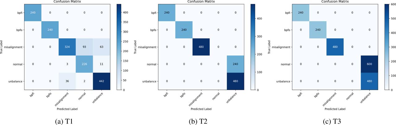
Fig. 2.
Confusion matrices of the proposed model under the three transfer tasks.
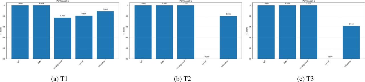
Fig. 3.
Per-class F1 scores of the proposed model under the three transfer tasks.
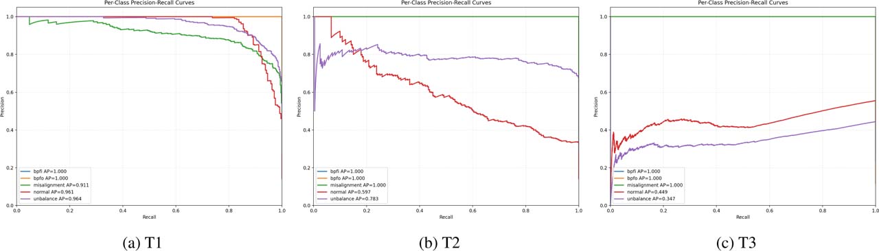
Fig. 4.
Per-class precision–recall curves of the proposed model under the three transfer tasks. AP denotes average precision.
T2 and T3 show a more specific failure mode. BPFI, BPFO, and misalignment are classified perfectly, but all target normal windows are assigned to the unbalanced class. This yields normal F1=0 and reduces unbalanced F1 to 0.800 in T2 and 0.615 in T3. The PR curves reinforce this diagnosis: normal AP decreases to 0.597 and 0.449, while unbalanced AP decreases to 0.783 and 0.347. The larger T3 normal set (600 windows) also explains why this single confusion pattern depresses its overall accuracy more strongly. These class-wise results prevent the aggregate metrics from obscuring a practically important healthy/fault ambiguity.
D. Feature-space visualization
Fig. 5 visualizes source-validation and target-test fused features. Across the three tasks, BPFI, BPFO, and misalignment generally form class-specific regions, consistent with their strong F1 values. The T2 and T3 embeddings show pronounced overlap between normal and unbalanced target features, matching the confusion matrices and PR curves. T1 has less severe overlap for these classes and consequently produces the best macro-F1. Because t-SNE preserves local neighborhoods but can distort global distances, the plots are treated as qualitative support rather than a quantitative measure of domain alignment.
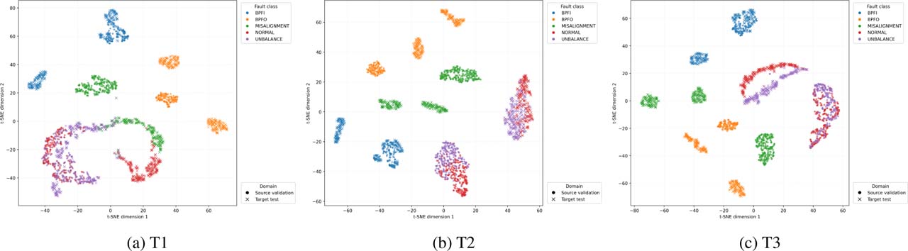
Fig. 5.
t-SNE visualization of fused source-validation (circles) and target-test (crosses) features. Colors denote fault classes.
4. Discussion
The external comparison and ablations provide complementary evidence. The proposed architecture is not simply a larger classifier: removing domain alignment (A4) causes the largest average loss, and replacing MK-MMD with a single kernel (A5) is particularly harmful in T1 and T2. Meanwhile, the mixed behavior of A1–A3 across tasks indicates that STFT and FFT contribute differently depending on transfer direction. The adaptive gate is therefore useful at the aggregate level because it avoids imposing one fixed representation balance on all samples, while the fused-space alignment provides the most consistent protection against load-induced shifts.
The result pattern also explains why the proposed model improves the task average without winning every individual metric. ACDANN achieves higher T2 macro-F1, and MSSA ties the proposed T2 accuracy; both explicitly emphasize domain or subdomain matching. The proposed method gains more on T1 and T3 because its same-segment dual representation provides complementary local and global evidence prior to alignment. In contrast, IRDDDA was originally designed around class imbalance and iterative classifier recalibration; under the present multi-source load-transfer setting, its adapted implementation does not transfer as effectively.
The main limitation is the normal–unbalanced ambiguity in T2 and T3. File-level separation is essential for avoiding leakage between windows from the same recording, but only one normal file is available per load. Hence, no normal windows are present in the target-unlabeled training subset, and distribution matching cannot directly observe that target class. The t-SNE overlap and zero normal F1 are consistent with this data constraint. Further experiments should collect multiple independent normal recordings per condition, adopt group-stratified splits when such recordings become available, evaluate repeated random seeds, and test transfer across speeds, sensors, and machines.
5. Conclusion
A cross-condition vibration-diagnosis framework that combines same-segment STFT/FFT representations, heterogeneous CNN–TCN encoding, adaptive gated fusion, and fused-space MK-MMD alignment has been evaluated across all three many-to-one load-transfer tasks. The task results are 87.62/89.24 %, 85.71/76.00 %, and 70.59/72.31 % in accuracy/macro-F1 for T1–T3. Compared with four external methods, the proposed model provides the highest task averages (81.31 % accuracy and 79.18 % macro-F1). A1–A5 ablations identify domain alignment as the most consistent contributor and show aggregate benefits from adaptive fusion and multi-kernel matching. Class-level and t-SNE analyses also reveal that the remaining performance loss is concentrated in normal–unbalanced separation when the unlabeled target split contains no normal recording. The framework is therefore effective across multiple load-transfer directions, while broader recordings are still necessary for stronger deployment evidence.
Acknowledgment
The authors gratefully acknowledge the public rotating machinery dataset providers for making the experimental data available. This work was supported by the 2024 Major University-Level Scientific Research Project of Liuzhou Polytechnic University, “Research and Development of a Large-Model-Based Spindle Fault Early Warning System for Automotive Transmission Machining Production Equipment” (Project No. 2024KA02), and by the 2024 Liuzhou Science and Technology Plan Project, “Research and Development of a Large-Model-Based Fault Early Warning System for Automotive Transmission Machining Production Equipment” (Project No. 2024AB0101A001).