
1. Introduction
Iron is the most important trace element, playing a critical role in a wide range of biological processes in the human body, including oxygen transport, cellular respiration, and enzymatic reactions. Iron homeostasis in the body is tightly regulated by the coordinated activity of specific metalloproteins, including hemoglobin, myoglobin, and ferritin. While hemoglobin in erythrocytes and myoglobin in muscle tissue provide reversible binding and transport of oxygen, ferritin serves as the primary intracellular reservoir for the safe storage of this potentially toxic metal. Abnormalities in the concentrations of these proteins directly correlate with various pathological conditions, from iron deficiency anemia to severe organ damage caused by iron overload (hemochromatosis) [1].
The magnetic properties of these metalloproteins are determined mainly by the oxidation and spin states of iron. Hemoglobin and myoglobin contain heme with a single Fe2+ atom and exhibit variable magnetic behavior: in the deoxygenated form (deoxy-state), they are paramagnetic due to the presence of unpaired electrons, while after binding oxygen (oxy-state), they transition to a diamagnetic configuration. The most complex response is represented by ferritin, whose core (6–7 nm) is formed by the nanocrystalline mineral ferrihydrite [2]. Due to the size of the antiferromagnetic ferrihydrite particles in the core, ferritin exhibits superparamagnetic behavior.
When analyzing complex biological matrices such as whole blood or tissue samples, the total magnetic susceptibility of the sample behaves as an additive system. The resulting magnetization is a linear superposition of the individual contributions: the diamagnetic background of water and cellular structures, the weak diamagnetic or paramagnetic contribution of transport proteins, and the dominant temperature-dependent response of ferritin core [3]. Understanding and separating these individual magnetic components is crucial for the quantitative interpretation of the measurements. The present work focuses on the systematic measurement and analysis of the magnetic properties of hemoglobin, myoglobin, and ferritin in defined concentration ranges. It also demonstrates the combination of contributions from individual iron-containing proteins into the resulting magnetization of the sample.
2. METHODS
Sample preparation
Available protein preparations were used (Sigma-Aldrich, USA): Hemoglobin human – lyophilized powder H7379 (Batch No. SLCR3463, 2023), Myoglobin from equine heart – lyophilized powder M1882 (Batch No. 0000389005, 2021), and two batches of Ferritin from equine spleen – saline solution (0.15 M sodium chloride solution) F4503 (Ferritin 1: Batch No. SLBZ5776, 2018, 63 mg/ml and Ferritin 2: Batch No. 0000486173, 2025, 80 mg/ml).
For the measurement of individual protein preparations, hemoglobin and myoglobin powders were dissolved in deionized water as follows: 20 µg of powder in 20 µl of water. Solutions were homogenized in an ultrasonic bath. Then 20 µl of solution was pipetted onto an 18 cm long and 6 mm wide strip of paper [4] in the form of a small drop and air-dried for 24 hours. Ferritin solutions were used as delivered and also pipetted onto the center of an 18 cm long, 6 mm wide V-shaped strip of paper as a 20 µl drop and air-dried for 24 hours. After drying, the samples were weighed and placed in a standard straw used in magnetometer, and then measured.
For measurement of concentration models, solutions from the powders were prepared as follows: hemoglobin and myoglobin – 25 mg of powder was dissolved in 0.3 ml of deionized water. Models were prepared by placing a piece of cotton wool weighing approximately 4 mg into the center of an 18 cm long enameled copper wire with a diameter of 0.2 mm. Prepared protein solutions and ferritin solutions were transferred to the models using a pipette with a volume set from 5 to 50 µl so that the resulting concentration corresponded to the desired concentration. The models were then air-dried for 24 hours at room temperature, dry weights were recorded, and used together with the weight of the cotton wool to calculate the protein concentration in the model. Typical model dimensions are 2 mm in diameter and 6 mm in length. They were placed in a standard straw used in magnetometer and then measured. Each model was prepared and measured three times.
The strip of paper, copper wire, and straw are diamagnetic and long enough to have a negligible output signal to the measured magnetic moment [5].
SQUID magnetometry
Magnetic properties of prepared samples and models were measured by the Quantum Design MPMS XL-7 AC SQUID magnetometer. The measurement protocol included: measurement with reciprocating sample option, 4 cm scan length, centering to the peak signal, 5 cycles, 2 scans per measurement, frequency 1.5 Hz, 2 measurements per one measurement point, and setting the field in no-overshoot mode. Suppression of the influence of water, salt, cotton wool, and protein coating on the resulting magnetization was also considered, and the best option seems to be a combination of drying the samples, which minimizes the influence of water, and subtracting the diamagnetism that comes from the protein coating, residual water, salt, and cotton wool. DC magnetization M(H) measurement at 300 K and up to 1 T field was chosen to determine the diamagnetic correction for each sample and model. Then the samples and models were measured at 2 K up to 7 T field, and the corresponding diamagnetic correction was subtracted from each measured curve. The data were then normalized to the dry weight of the samples or model. Measured dependences were analyzed, and to determine the Coercivity (HC) and Remanent magnetization (MR) as intersections of the H and M axes, respectively, a linear fitting between the two closest measured points to the given axis was used. Maximal magnetization (MMAX) was chosen as a parameter replacing the Saturation magnetization (MS), since the investigated materials do not experience saturation but appear to be combined systems with paramagnetic and ferromagnetic components. The mean values of HC, MR, and MMAX are plotted as points in the figures.
3. Results
M(H) dependences for all of the preparations and cotton wool, measured at 300 K, are shown in Fig. 1. Hemoglobin and myoglobin preparations showed almost identical diamagnetic slope, indicating that the protein base of both preparations is magnetically very similar. On the other hand, ferritin preparations are paramagnetic, and their curves differ, mainly due to the different properties of the iron in the core. Cotton wool, which was later used as a model base, also exhibits diamagnetism. Measured diamagnetism was used for the diamagnetic correction of 2 K curves of M(H) dependences, which can be seen in Fig. 2. Hemoglobin and myoglobin have very similar magnetic properties due to heme content (Fe2+), and their curves almost overlap. Both ferritin samples exhibit wide hysteresis, due to stronger interatomic interactions in the ferritin core. Ferritin 1 has a higher MMAX; on the other hand, there is a higher HC for Ferritin 2. This is most probably caused by different mineral sizes in the core. The summarized properties of the preparations are in Table 1.
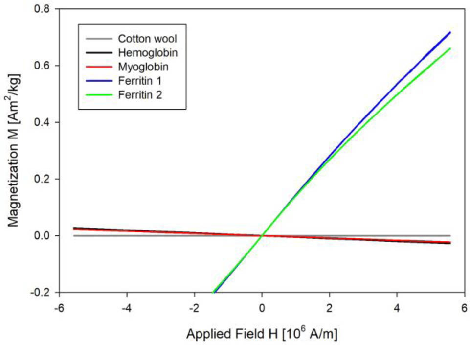
Fig 1.
M(H) dependences of cotton wool, hemoglobin, myoglobin, and ferritin preparations measured at 300 K.
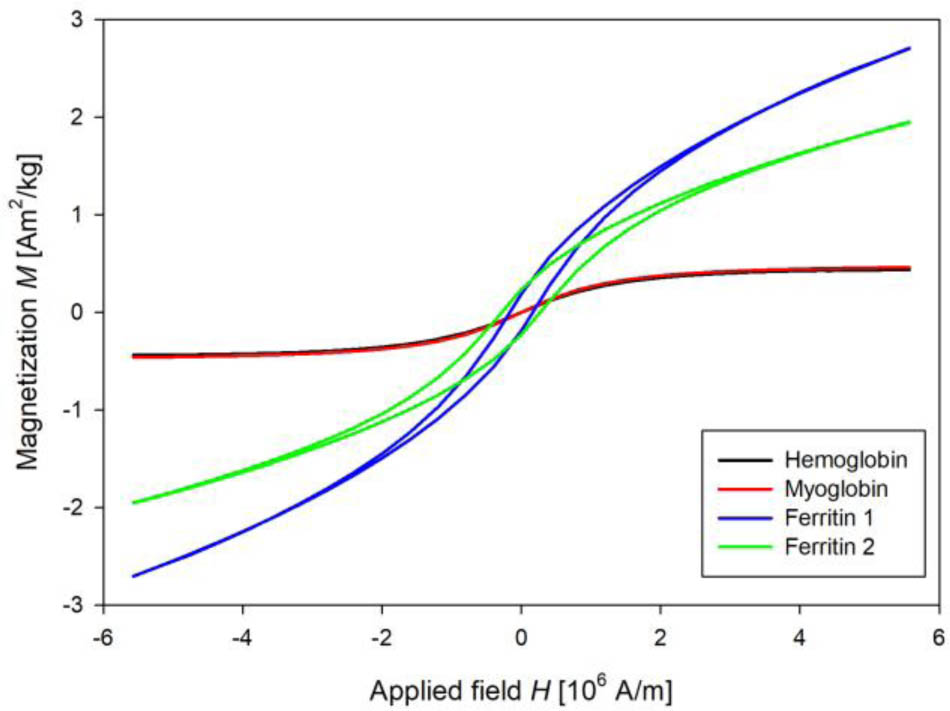
Fig 2.
M(H) dependences of hemoglobin, myoglobin, and ferritin preparations measured at 2 K after the diamagnetic corrections.
Table 1.
Derived parameters from M(H) dependences of protein preparations measured at 2 K.
| HC [A/m] | MR [10−3Am2/kg] | MMAX [Am2/kg] | |
|---|---|---|---|
| Hemoglobin | 1702 ± 81 | 0.49 ± 0.03 | 0.44 ± 0.21 |
| Myoglobin | 1032 ± 69 | 0.32 ± 0.02 | 0.46 ± 0.22 |
| Ferritin 1 | 164561 ± 8240 | 188.03 ± 9.51 | 2.71 ± 0.12 |
| Ferritin 2 | 275173 ± 14520 | 231.50 ± 10.25 | 1.95 ± 0.98 |
From these measurements, it can be concluded that heme proteins and ferritin have an irreplaceable influence on the magnetic properties of biological samples. Based on the known values of hemoglobin content in rat blood as 100 to 170 g/l (0.5 to 0.85 g of hemoglobin per gram, dry weight) [6], it was decided to create concentration models in the concentration range from 0.1 to 0.9 g of protein per gram of the model dry weight (C [gPT/g]).
Fig. 3(a) represents the dependence of HC on C. It can be seen that a change in C has almost no effect on HC and is without any indication of a trend over the entire measured range. Remanent magnetization is another parameter that defines the magnitude of hysteresis, and its dependence on concentration is shown in Fig. 3(b). MR clearly tracks the increase in C as its value increases for each protein, although linear regression of the data shows that this dependence does not start from zero. Fig. 3(c) shows the dependence of MMAX on C. From the linear regression curves, one can observe the dependence of magnetization on concentration. However, the dependences of all three quantities on concentration for hemoglobin and myoglobin are almost identical because they contain the same prosthetic group – heme containing one iron atom (Fe2+). On the other hand, there are different dependencies for both ferritin proteins, probably due to differences in iron loading and core mineral size.
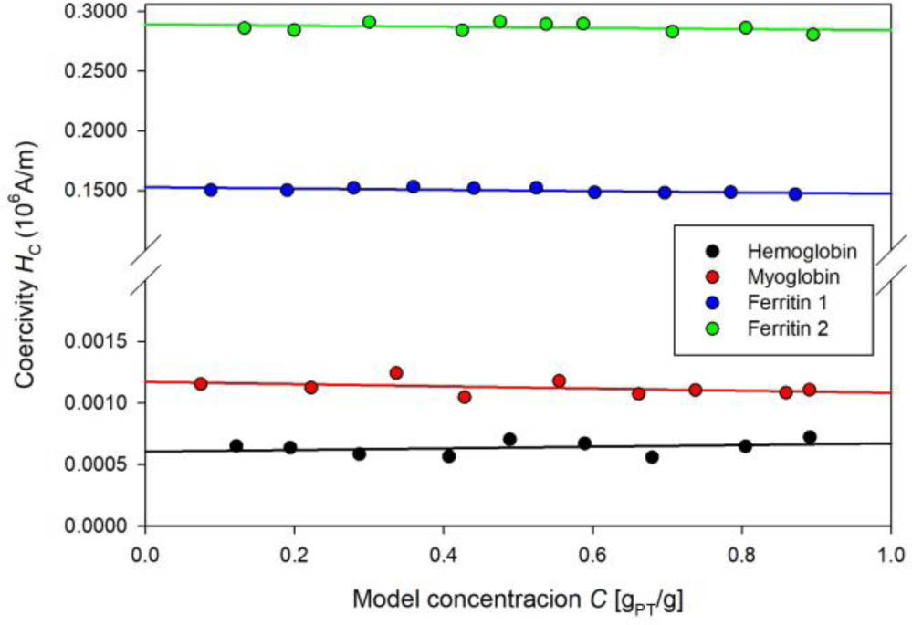
Fig. 3(a).
HC vs C for hemoglobin, myoglobin, and ferritin concentration models. SD of HC is 80, 83, 2400, and 2940 for hemoglobin, myoglobin, ferritin 1, and ferritin 2 models. The straight lines represent a linear regression of the measured data for each model (R2 = 0.092, 0.178, 0.433, 0.117, with slope 66, −88, −5431, −4975 and intercept 604, 1170, 152738, 289016).
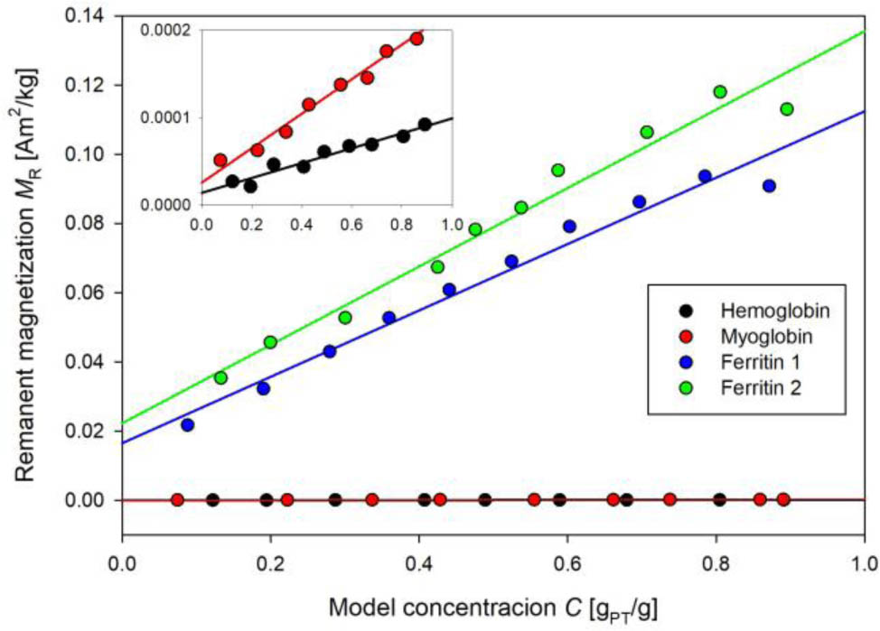
Fig. 3(b).
MR vs C for hemoglobin, myoglobin, and ferritin concentration models. SD of MR is 4.6 × 10⁻⁶, 5.1 × 10⁻⁶, 5.5 × 10⁻⁴, and 5.4 × 10⁻⁴ for hemoglobin, myoglobin, ferritin 1, and ferritin 2 models. The lines are a linear regression of the measured data for each model (R2 = 0.943, 0.979, 0.974, 0.970 with slope 8.5 × 10⁻⁵, 1.9 × 10⁻⁴, 9.6 × 10⁻², 11.3 × 10⁻² and intercept 1.4 × 10⁻⁵, 2.58 × 10⁻⁵, 1.6 × 10⁻², 2.2 × 10⁻²).
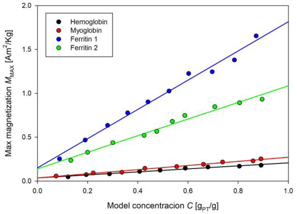
Fig. 3(c).
Dependence of MMAX vs C for hemoglobin, myoglobin, and ferritin concentration models. SD of MMAX is 9.6 × 10⁻³, 8.6 × 10⁻³, 1.6 × 10⁻³, and 1.8 × 10⁻³ for hemoglobin, myoglobin, ferritin 1, and ferritin 2 models. Lines are a linear regression of measured data for each model (R2 = 0.978, 0.986, 0.987, 0.980 with slope 17.1 × 10⁻², 23.5 × 10⁻², 1.67, 0.95 and intercept 3.5 × 10⁻², 3.6 × 10⁻², 15.0 × 10⁻², 13.9 × 10⁻²).
It is well known that individual magnetic contributions add to the resulting magnetization according to the principle of superposition [3], [7]. It can therefore be stated that similarly, the contributions of individual iron-containing proteins add up to the resulting magnetization of a real biological sample. It is possible to present a model case (Fig. 4) of such a result, given that the sample contains hemoglobin and myoglobin at a concentration of 0.1 gPT/g and both ferritins at a concentration of 0.05 gPT/g. As can be seen, for maximum magnetization, a simple summation of individual contributions is valid, but the coercivity and remanent magnetization values carry the shape component of individual curves. Derived parameters for this resulting curve are:
HC = 138 800 A/m,
MR = 0.0348 Am2/kg, and
MMAX = 0.5372 Am2/kg.
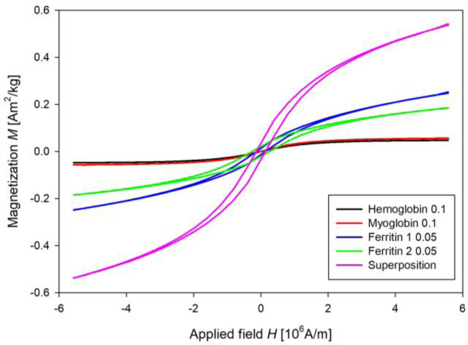
Fig. 4.
Superposition of individual proteins into the resulting curve. Simulated concentration of 0.1 gPT/g was used for hemoglobin and myoglobin, and 0.05 gPT/g was used for both ferritin preparations.
4. Conclusions
The SQUID magnetic measurements showed that heme proteins and ferritin have different profiles. Thanks to this, it is expected that it will be possible to magnetometrically determine not only the amount of iron in animal samples but also its incorporation into iron-containing proteins. Concentration model measurements showed that the relationships of individual derived parameters of hysteresis loops measured at 2 K, except for coercivity, are linearly dependent on the concentration of individual proteins in the model. On the other hand, the preservation of information in the loop width by a given coercivity shows that even with this value, it is possible to detect the presence of various proteins in the sample. However, for the coercivity alone, one cannot simply use the superposition of individual proteins as for the maximum magnetization, because the shape of the curve is also crucial. The model case with a combination of proteins showed that it is possible to combine the measured M(H) curves from contributions of individual proteins to the resulting curve. It is assumed that analyzing the shape of the measured M(H) curve, combined with knowledge of concentration dependencies, could enable decomposition of this curve into contributions from individual proteins in real samples.
Acknowledgements
This work was funded by the EU NextGenerationEU through the Recovery and Resilience Plan for Slovakia under the project No. 09I03-03-V04-00528.