
1. Introduction
The mathematical pendulum is a widely accepted model of nonlinear oscillators, occupying a pivotal position in both fundamental physics and applied engineering [1]. The simplicity of its structure — consisting of a mass suspended by a massless, inextensible string — and its inherent nonlinear dynamics, governed by equations involving trigonometric nonlinearities, make it a cornerstone for studying complex phenomena such as amplitude-dependent frequency, nonlinear resonance, and even chaotic behavior [2]. Beyond its role in validating nonlinear vibration theories, the mathematical pendulum serves as a prototype for understanding more intricate systems, with applications spanning from classical mechanics to cutting-edge micro/nanoengineering [3]–[5].
In the domain of Micro-Electro-Mechanical Systems (MEMS) [4]–[6], the principles of the mathematical pendulum and the Duffing oscillator are of particular significance. These principles underpin the design and operation of critical devices. For instance, MEMS accelerometers and gyroscopes leverage pendulum-like proof masses and oscillating structures to achieve high-precision motion sensing, where nonlinear dynamics directly influence sensitivity and stability [7]. The ability to model and predict the nonlinear behavior of such miniaturized pendulum systems is thus essential for advancing MEMS technology, from inertial navigation to IoT sensors [8], [9].
Nevertheless, the resolution of the nonlinear vibration problem of the mathematical pendulum remains a significant challenge. Conventional analytical methods often fail to yield closed-form solutions, a consequence of the system's inherent nonlinearity. Moreover, numerical approaches are susceptible to computational inefficiency or sensitivity to initial conditions. In addressing this issue, various approximation methods have been developed over the years. These include the homotopy perturbation method (HPM) [10], [11] and the variational iteration method [12], which have been proven to be powerful tools for tackling strongly nonlinear systems. The HPM method, for instance, has been used in the context of non-conservative oscillators, offering approximate solutions by decomposing complex problems into more manageable subproblems [13]. Furthermore, the variational iteration method has been used to analyze nonlinear oscillations, thereby offering insights into dynamic responses through iterative corrections [12]. However, these methods continue to face limitations in terms of balancing accuracy, computational efficiency, and adaptability to diverse boundary conditions, particularly in context-specific applications such as MEMS systems [14], [15].
In light of the aforementioned context, He's frequency formulations [16]–[18] have emerged as a promising alternative, providing a robust framework for the simplification of nonlinear vibration analysis while maintaining precision. These models have found wide applications in engineering, as evidenced by Zhang et al. [19], who provided a comprehensive analysis of He's frequency formulation applied to fractal-fractional nonlinear oscillators. Niu et al. [20] explored the contemporary applications of ancient mathematics with a particular emphasis on He's frequency formulation for MEMS systems. Mohammadian [21] applied his recently developed frequency-amplitude formulation to nonlinear oscillators. This was achieved by introducing a novel approach for determining location points. Zhang et al. [22] conducted a study into the application of He's frequency formula to nonlinear oscillators under generalized initial conditions. Feng [23] applied the formulation to vibration systems in porous media. He et al. [24] demonstrated the effectiveness of the frequency formulation in analyzing the pull-down instability of nonlinear oscillators. Feng [25] studied the fractal undamped Duffing oscillator and further extended it to nonlinear vibrations of porous foundations [26] and fractal vibration systems [27]. Many modifications have emerged, among which those by Chun-Hui He and his colleagues have significantly enhanced mathematical rigor and accuracy [28]–[30].
The present study builds on this progress by applying an improved frequency formulation to the mathematical pendulum, aiming to complement existing analytical methods and enhance their applicability to practical scenarios, including MEMS-related dynamics. The main objective is to derive reliable numerical solutions for the nonlinear vibrations of the pendulum using the modified frequency formulation, with particular attention to the strategic selection of location points. The motion equation is transformed into a form compatible with the formulation, and case-specific derivations are conducted for three distinct location point configurations. The numerical solutions and visualizations are analyzed to reveal how different location point settings influence the dynamic behavior. These findings contribute to a better understanding of pendulum-based systems and may offer useful guidance for the design of MEMS devices and related applications.
The structure of the paper is as follows: Section 2 focuses on fundamental theory and formula derivation, including the nonlinear oscillator model, the modified frequency formulation, and the derivation of the key equations for the mathematical pendulum. Section 3 presents a detailed analysis of numerical solutions for three distinct location point configurations, and for each configuration, the derived frequency formulation is discussed. Section 4 presents comparison results and a discussion of the modified frequency formulation with classical analytical methods and numerical solutions, analyzes the relative errors across different amplitude ranges, and verifies the advantages of the proposed method. Finally, Section 5 summarizes the key findings, confirms the applicability of the modified frequency formulation for solving the nonlinear vibration problem of the mathematical pendulum, and outlines the limitations of the current study and directions for future work.
2. Fundamental theory and formula derivation
A. Nonlinear oscillator model
Nonlinear oscillators, characterized by amplitude-dependent dynamic behavior and trigonometric or polynomial nonlinearities, are fundamental components of numerous physical and engineering systems. This paper considers the differential equation of a nonlinear oscillator given by
These systems range from classical mechanical pendulums to miniaturized MEMS resonators [3], [7], [19]. As previously mentioned in Section 1, the mathematical pendulum serves as a paradigmatic example of such systems, governed by nonlinear differential equations that resist closed-form solutions via traditional analytical methods. To address this challenge, a generalized nonlinear oscillator model, expressed as follows, serves as the foundational framework for the present study.
where ü represents the second derivative of the displacement with respect to time, and denotes the nonlinear restoring force term. This model encapsulates the essential dynamic features of nonlinear vibrational systems, including the mathematical pendulum, making it a suitable starting point for deriving problem-specific solutions.Conventional approximation methods (e.g., homotopy perturbation or variational iteration methods) face limitations in balancing accuracy and efficiency, particularly in context-specific applications such as MEMS [14], [15]. The modified frequency formulation proposed by Chun-Hui He and colleagues [29], [30] emerges as a refined analytical tool. This enhanced framework builds on the original frequency formulations developed by Ji-Huan He [16]–[18], enhancing mathematical rigor and adaptability to diverse nonlinear systems, including those with complex boundary conditions or fractal characteristics [28]. The core of the modified frequency formulation is given by:
where ω denotes the angular frequency of oscillation, a2k+1, k = 0, …, N are constants, and ū2k+1, k = 1, …, N are location points. This modification addresses the key drawbacks of earlier methods, such as sensitivity to initial conditions and limited precision in high-amplitude vibrations. These are critical for applications such as MEMS gyroscopes, where precise frequency prediction directly affects sensing accuracy [7], [8].A distinguishing characteristic of the modified frequency formulation is its reliance on “location points” to tailor the general framework to specific systems. As established in [29], location points are defined as:
In the context of the mathematical pendulum, these location points assume a pivotal role in the transformation of the generalized oscillator model (2) into a form that reflects the pendulum's unique nonlinearity (i.e., the sine-term restoring force). By strategically setting location points, the formulation gains flexibility to accommodate a range of physical scenarios — from small-angle approximations to large-amplitude oscillations — thus bridging theoretical generality and problem-specific accuracy.
In summary, the nonlinear oscillator model (2) provides a universal description of nonlinear vibrations, while the modified frequency formulation (3) offers a robust solution tool, and the location points (4) enable its application to the mathematical pendulum. The tripartite framework serves as the foundation for deriving the pendulum's motion equation in part B of Section 2, ensuring both theoretical consistency and applicability to practical scenarios, such as MEMS dynamics.
B. Modified frequency formulation of a simple mathematical pendulum
The dynamic behavior of a simple mathematical pendulum is attributed to the interplay between the gravitational force and the constraint imposed by its massless, inextensible string, resulting in inherently nonlinear motion. The motion of the simple mathematical pendulum is given by
where A is the amplitude.The nonlinear term introduces strong nonlinearity, as its trigonometric nature prevents the equation from yielding closed-form solutions via traditional linear methods – especially for large-amplitude oscillations, which are critical in practical scenarios such as MEMS accelerometers where nonlinearity directly affects sensitivity [7], [8].
In order to leverage the modified frequency formulation (3) introduced in part A of Section 2, the original equation (5) must be transformed into a form that is compatible with the structure of generalized nonlinear oscillator models (2). This transformation focuses on reorganizing the nonlinear term to align with the analytical framework of the modified frequency formulation, while preserving the physical essence of the pendulum's dynamics.
To facilitate the application of the modified frequency formulation, (5) is transformed into a more suitable form
where , , .This transformed form (6) achieves two critical objectives:
The model under consideration aligns with the general structure of nonlinear oscillator models (2), in which the nonlinear restoring force F(u) = sinu is clearly identified. This enables direct integration with the modified frequency formulation (3).
The model employs a Taylor expansion of the sinusoidal nonlinearity up to the seventh order, yielding a seventh-degree polynomial approximation. This truncation order is chosen because it provides a good balance between accuracy and algebraic simplicity for amplitudes up to A = 3. This approximation retains the essential nonlinear characteristics of the original system for moderate-to-large oscillation amplitudes and provides superior accuracy compared to the conventional small-angle approximation sinu ≈ u. This ensures the model remains valid for large-amplitude oscillations, a prerequisite for analyzing real-world systems such as MEMS resonators, where significant displacements often occur [4], [6].
Preserving the physical nonlinearity while refining the mathematical structure is paramount for this transformation, as it provides a rigorous foundation for the subsequent integration with the modified frequency formulation. This integration facilitates the derivation of problem-specific equations in part C of Section 2 and enables tailored analysis under different location point settings.
To integrate the transformed motion equation of the mathematical pendulum with the modified frequency formulation, by employing algebraic manipulation and substituting the variable defined in part A of Section 2, the specific form of the modified frequency formulation of the mathematical pendulum's motion is given in (7):
This equation serves as the key analytical basis for the case-specific derivations in the subsequent sections, enabling the exploration of the pendulum's nonlinear vibration characteristics under different location point settings.
3. Numerical solution under different location point configurations
A. First location point setting: Fixed location point
In this case, the fixed location point (FLP) is specifically chosen as
This setting serves as a critical reference for deriving the motion equation of the mathematical pendulum under the corresponding conditions. Based on the location point given in (8), combined with the fundamental framework of the modified frequency formulation (7), the corresponding frequency formulation for this scenario is derived as
and the approximate solution is expressed byB. Second location point setting: Incorporating adjustable parameter k
For the second case, the location point with parameter k (kLP) is defined as
where k is a parameter that needs to be determined. We consider the parameter to be related to amplitude A. A key difficulty in using the frequency formulation is selecting a proper value for the location point [21]. It is better to describe the value of k as a function that depends on both the amplitude and system parameters. This distinct setting differentiates it from the first cases, aiming to explore how a varied reference point influences the pendulum's motion.To determine the magnitude of k, (1) can be rewritten as follows
where .If the frequency derived from (3) is taken as the exact frequency, the right-hand side of (12) will become zero. By applying the Galerkin technique and using cos(ωt) as the weighting function, the following equation is obtained
where . For the present problem, (12) can be rewritten as:If the frequency derived from (9) counts as the exact frequency, the right-hand side of (14) will go to zero. Based on (13), we obtain:
Substituting u = Acos(ωt) into (15), we get the equation in the form as follows
Substituting the values of β1, β2 and β3 into (16) yields
Let k2 = X, then (17) can be transformed into
X can be obtained using the root-finding formula for cubic equations, and further, we can determine the parameter k, which is related to amplitude A. By substituting the value of k into (11), the approximate frequency ωkLP is determined using (7) as follows
and the approximate solution is expressed byIt is worth noting that although the parameter k can be solved via cubic equation root-finding after variable substitution, this process still requires complex algebraic operations, including square root and cube root calculations. It does not provide a significant computational advantage over the fixed-step fourth-order Runge-Kutta (RK4) method.
C. Third location point setting: Modified location point
The third scenario adopts a modified location point (MLP) definition obtained from (4) as follows:
This setting further expands the scope of investigation, offering another perspective to examine the mathematical pendulum's nonlinear vibrations. Building on the location point defined in (20), the modified frequency formulation for this case is derived as
and the corresponding approximate solution is expressed byBy applying the modified frequency formulation (3) and the transformed pendulum motion equation (6), this derivation follows the consistent logic of adapting the frequency formulation to specific location points, yielding an equation that reflects the unique characteristics of this setting.
4. Comparison results and discussion
To comprehensively validate the performance of the modified frequency formulation in solving the nonlinear vibration problem of the mathematical pendulum, we systematically compare its results with those obtained from classical analytical methods and numerical solutions. The classical analytical methods selected for comparison include the HPM, the modified homotopy perturbation method (MHPM), and the harmonic balance method (HBM), which are widely recognized for their applicability to nonlinear oscillators. The numerical solution, obtained via the fourth-order Runge-Kutta (RK4) method, serves as the benchmark for evaluating accuracy, given its high precision in solving differential equations.
To apply the RK4 method, the second-order ODE (1) is converted into an equivalent system of two first-order ODEs. Define the state variables
Differentiating these gives the system
and the initial conditions becomeWe use a fixed time step Δt = 0.001 and let tn = n · Δt, u1,n ≈ u(tn), and u2,n ≈ u̇(tn). The goal is to compute u1,n+1 and u2,n+1 from u1,n and u2,n according to the following procedure:
whereThe HPM is a prominent analytical technique for nonlinear systems, particularly effective when traditional linearization or closed-form solutions is unattainable [10], [11]. Its core principle is to construct a homotopy function that deforms a solvable linear system into the target nonlinear system, using a perturbation parameter to approximate the solution through series expansion. This method avoids reliance on small parameters, a limitation of classical perturbation methods, and balances accuracy with computational efficiency, making it suitable for strongly nonlinear systems like the mathematical pendulum described by (5).
For comparative purposes, we adopt representative period approximations from the existing literature for HPM, MHPM, and HBM. For example, the approximate period of the mathematical pendulum derived via HPM in [31] is given by:
where .The second-order approximate period from the standard HPM in [32] is presented as:
The approximate period obtained via MHPM in [33] is shown as:
The second-order approximate period from HBM in [34] is given by:
Table 1 summarizes the periods and their relative errors, calculated using the three types of location point configurations alongside the four aforementioned analytical methods. The relative error is defined as:
where r = FLP, kLP, MLP, HPM1, HPM 2, MHPM, HBM, TRK denotes the period from the RK4 numerical solution, and Tr represents the period from other analytical methods. The periods for the three location point configurations are calculated as , and .As shown in Table 1, the performance of these methods varies significantly across different amplitude ranges, reflecting the influence of nonlinearity intensity on the computational accuracy.
Table 1.
Comparison of periods and their relative errors obtained from various methods.
| A | TRK | TFLP Err(%) | TkLP Err(%) | TMLP Err(%) | THPM1 Err(%) | THPM2 Err(%) | TMHPM Err(%) | THBM Err(%) |
|---|---|---|---|---|---|---|---|---|
| 0.1 | 6.2871 | 6.2871 | 6.2871 | 6.2871 | 6.2871 | 6.2871 | 6.2871 | 6.2871 |
| 0.0000 | 0.0000 | 0.0000 | 0.0000 | 0.0000 | 0.0000 | 0.0000 | ||
| 0.3 | 6.3187 | 6.3187 | 6.3187 | 6.3187 | 6.3187 | 6.3187 | 6.3187 | 6.3187 |
| 0.0001 | 0.0003 | 0.0002 | 0.0003 | 0.0000 | 0.0000 | 0.0003 | ||
| 0.5 | 6.3828 | 6.3827 | 6.3826 | 6.3829 | 6.3826 | 6.3828 | 6.3828 | 6.3827 |
| 0.0004 | 0.0024 | 0.0012 | 0.0022 | 0.0000 | 0.0000 | 0.0022 | ||
| 1.0 | 6.7000 | 6.6994 | 6.6975 | 6.7014 | 6.6961 | 6.6999 | 6.6999 | 6.6971 |
| 0.0085 | 0.0362 | 0.0206 | 0.0581 | 0.0018 | 0.0015 | 0.0429 | ||
| 1.4 | 7.1523 | 7.1493 | 7.1410 | 7.1583 | 7.1222 | 7.1504 | 7.1505 | 7.1372 |
| 0.0418 | 0.1588 | 0.0833 | 0.4202 | 0.0267 | 0.0249 | 0.2110 | ||
| 1.8 | 7.8582 | 7.8456 | 7.8173 | 7.8773 | 7.6987 | 7.8419 | 7.8424 | 7.7963 |
| 0.1592 | 0.5206 | 0.2441 | 2.0296 | 0.2075 | 0.2001 | 0.7869 | ||
| 2.0 | 8.3498 | 8.3249 | 8.2758 | 8.3820 | 8.0238 | 8.3083 | 8.3094 | 8.2303 |
| 0.2978 | 0.8853 | 0.3864 | 3.9041 | 0.4963 | 0.4832 | 1.4304 | ||
| 2.5 | 10.3232 | 10.1737 | 9.9878 | 10.4237 | 8.8029 | 9.9763 | 9.9805 | 9.7238 |
| 1.4480 | 3.2487 | 0.9735 | 14.726 | 3.3597 | 3.3193 | 5.8064 | ||
| 3.0 | 16.1555 | 14.2775 | 13.4646 | 15.7941 | 9.2483 | 12.7146 | 12.7271 | 12.0333 |
| 11.6246 | 16.6565 | 2.2371 | 42.7546 | 21.2986 | 21.2217 | 25.5159 |
In the amplitude range A ≤ 2, the system's nonlinearity is relatively small or moderate. Both the three location point configurations and traditional methods (e.g., optimized HPM variants, MHPM, HBM) can effectively capture the pendulum's vibration characteristics. For instance, at A = 0.1 and A = 0.3, all methods yield a period of 6.2871 and 6.3187, respectively, with relative errors as low as nearly zero. Even at A = 2, the relative errors of the three configurations remain less than 1 %, while those of optimized traditional methods, like standard HPM2 in [32] and MHPM in [33], are similarly low, reflecting high consistency and low deviations from numerical solutions. By contrast, the HPM in [31] and HBM in [34] exhibit higher relative errors of 3.9 % and 1.4 % under the same conditions. This collectively demonstrates the effectiveness of multiple approaches under mild nonlinearity. The deviations between their calculated results and numerical solutions remain at a low level, and there is overall high consistency among the methods.
When the amplitude reaches and exceeds 2.5, the system's nonlinearity intensifies sharply, with trigonometric nonlinearity dominating the pendulum's vibration. As Table 1 reveals, at this stage, the third configuration (modified location point) exhibits distinct advantages. Its improved design is uniquely adapted to dynamic balance under strong nonlinearity, as evidenced by its maximum relative errors of 0.97 % at A = 2.5 and 2.23 % at A = 3. The first and second location point configurations also exhibit higher errors than the third configuration, but their performance remains superior to that of other analytical methods. For instance, at A = 2.5, their errors are significantly lower than those of HPM in [31] and HBM in [34], and even slightly better than HPM2 in [32] and MHPM in [33]. At A = 3, their errors are much smaller than those of the other four analytical methods. This indicates that while the first and second location point configurations cannot prevent error growth under strong nonlinearity, they still outperform other traditional analytical methods in terms of accuracy. Compared to the first, second configuration, and traditional methods, the third location point configuration method approximates the numerical solution more stably, with better control over the magnitude and rate of error growth, and can more reliably reflect the pendulum's vibration characteristics under large amplitudes and strong nonlinearity, demonstrating the adaptability of the optimized location point method in strong nonlinear scenarios.
From a spectral perspective, the MLP method establishes an implicit connection with the HBM. While we assume a pure fundamental harmonic solution form u = Acos(ωt) for simplicity, the symmetric nonlinearity of the mathematical pendulum introduces significant third harmonic components in its actual vibration spectrum. The two-point configuration with a 12:1 weighting ratio can be interpreted as capturing the dominant nonlinear effect induced by the third harmonic component, and this physical interpretation is derived from the spectral feature of pendulum vibration, without a rigorous mathematical Fourier decomposition proof in this work. This method avoids explicit Fourier series expansion for high-order harmonics. This approach avoids the computational complexity of solving coupled algebraic equations for higher harmonics in traditional HBM while still capturing the dominant nonlinear effects through optimized location point selection. This spectral interpretation provides a deeper physical understanding of why the MLP method achieves superior accuracy in strongly nonlinear regimes.
In terms of practical engineering applicability, the explicit algebraic form of the MLP method represents a significant advantage over both the kLP method and traditional numerical solvers. In contrast, the MLP method provides a direct, closed-form calculation of the oscillation frequency, enabling its implementation on resource-constrained microcontrollers in MEMS sensors and other embedded systems. This combination of high accuracy and low computational cost makes the MLP method particularly valuable for real-time vibration prediction and control applications.
Fig. 1 visually presents the quantitative results in Table 1, providing intuitive insights into the performance of the three location point configuration methods compared to traditional methods. Fig. 1 illustrates the trend of relative errors for all evaluated methods as a function of amplitude A. For small amplitudes, all methods exhibit near-zero errors, with the error curves clustering near the horizontal axis. This confirms the consistency of all approaches under weak nonlinearity. As amplitude increases, the error curves diverge: traditional methods (HPM, MHPM, HBM) show steeper upward slopes, indicating rapid error accumulation. In contrast, the three location point configurations maintain gentler slopes, with the third configuration consistently lying below the first and second, reflecting its smaller error growth rate. At large amplitudes, the third configuration's error curve is distinctly lower than those of the traditional methods and the other two location point configurations, visually validating its superior stability in strongly nonlinear regimes.
Fig. 2 illustrates how parameter k varies with respect to amplitude A for the second studied case. As shown in the figure, parameter k decreases as amplitude A increases. This indicates that parameter k is related to amplitude A.
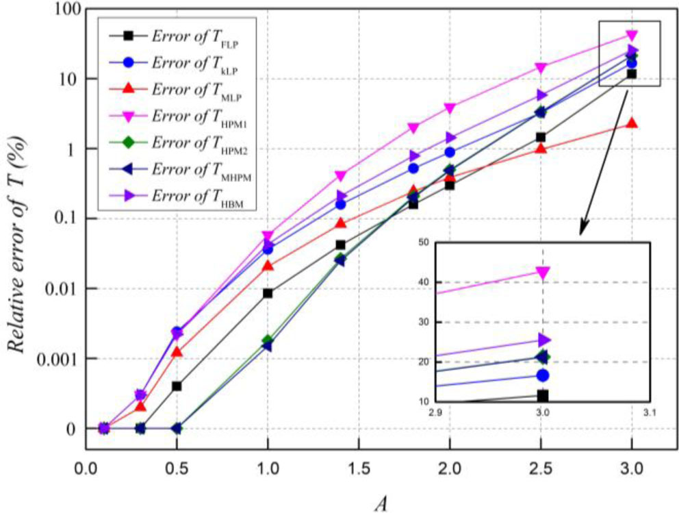
Fig. 1.
Comparison of the relative error with respect to amplitude for the different methods.
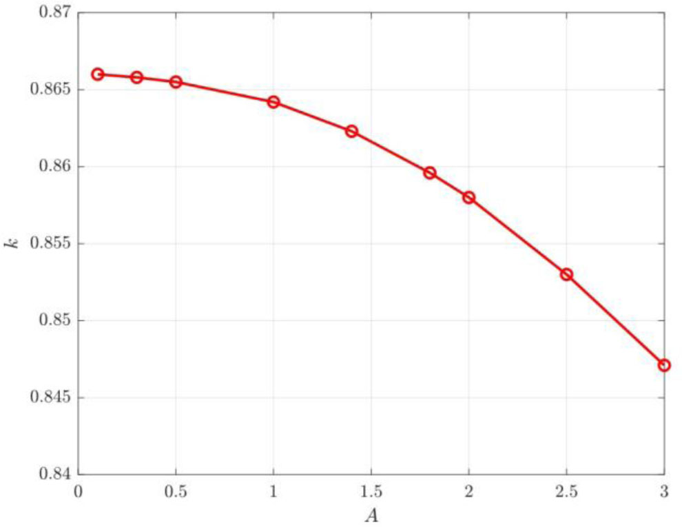
Fig. 2.
The variation of k with respect to amplitude A in the second location point configuration.
Fig. 3–Fig. 6 further compare the analytical solutions from the three location point configurations with the numerical solution across specific amplitudes of A = 0.1, 1, 2, 3. Fig. 3–Fig. 5 focus on comparing the analytical solutions from the three location point configurations with the numerical solution for the mathematical pendulum at small to moderate amplitudes. For the three location point configurations, their analytical solution curves overlap nearly completely with the numerical solution curve. This visual coherence confirms the quantitative findings in Table 1, where relative errors for these configurations remain low in this amplitude range, indicating their ability to accurately capture the pendulum's dynamic behavior when nonlinearity is not yet dominant. Fig. 6 focuses on the comparison under large amplitudes, where strong nonlinearity dominates the pendulum's vibration. In this regime, the figure clearly demonstrates the distinct advantage of the third location point configuration. While all analytical methods show increased deviation from the numerical solution due to the strong trigonometric nonlinearity, the third configuration's curve remains closest to the numerical solution. Compared to the first and second location point configurations, its deviation is noticeably smaller, aligning with Table 1's finding that it exhibits lower relative error in large-amplitude scenarios. The figure visually confirms that the third configuration avoids the larger divergences observed in traditional methods (as implied by Table 1's data on HPM, MHPM, and HBM), maintaining a more stable alignment with the numerical solution. This reflects its optimized location point design, which is better tailored to balance the dynamic characteristics of strong nonlinear vibrations.
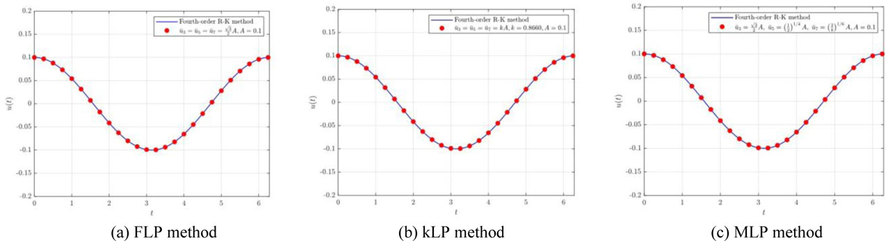
Fig. 3.
Comparing the analytical solutions with the numerical solution for the three types of location points with A = 0.1.
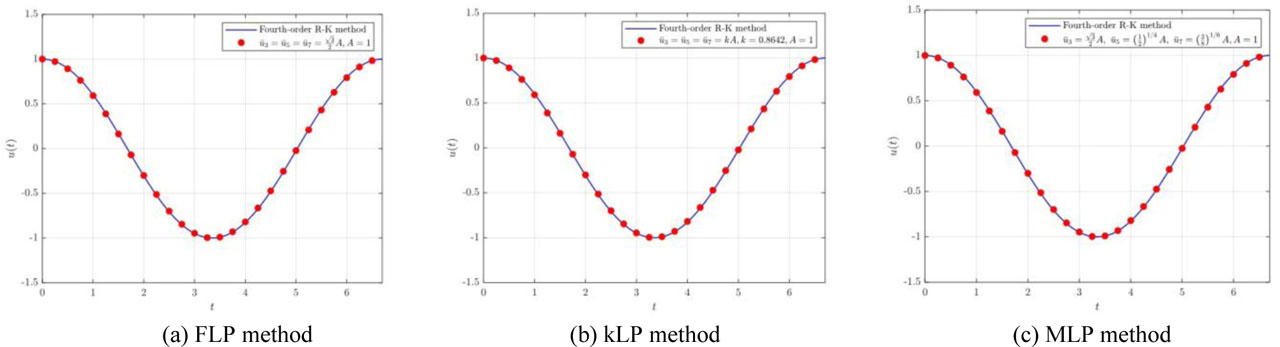
Fig. 4.
Comparing the analytical solutions with the numerical solution for the three types of location points with A = 1.
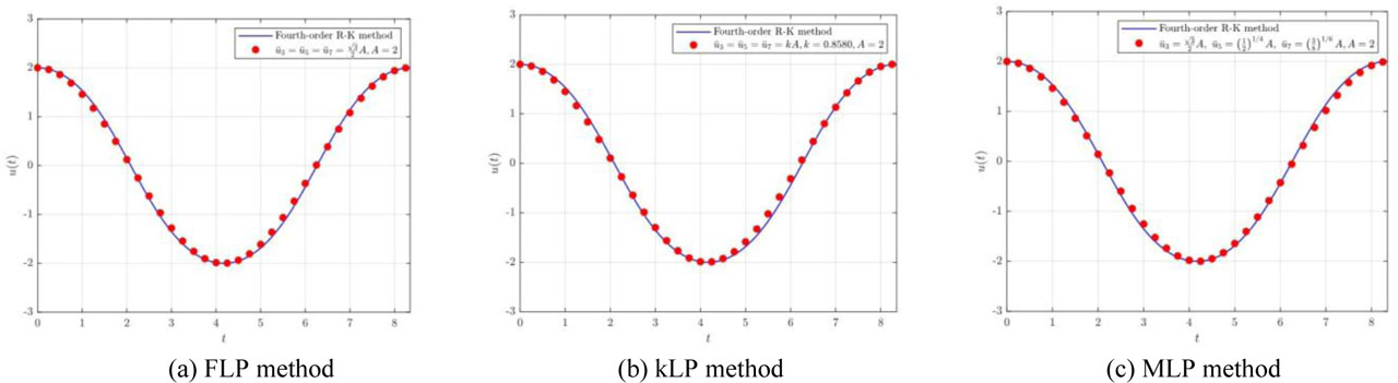
Fig. 5.
Comparing the analytical solutions with the numerical solution for the three types of location points with A = 2.
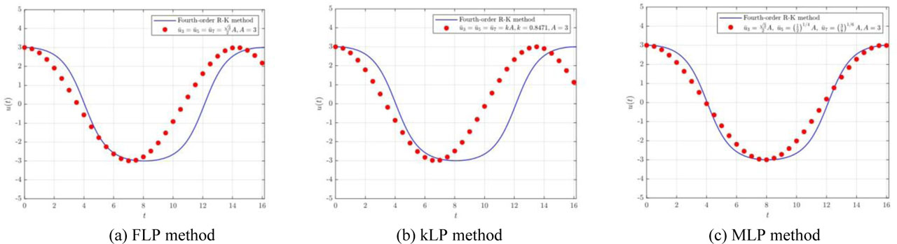
Fig. 6.
Comparing the analytical solutions with the numerical solution for the three types of location points with A = 3.
Overall, the modified frequency formulation with well-defined location points effectively captures the nonlinear vibration characteristics of the mathematical pendulum and delivers more stable calculation results with smaller error growth than most traditional analytical methods under large-amplitude, strong nonlinear vibrations. For small and moderate vibration amplitudes, the HPM and the HBM can also produce satisfactory approximate periods.
5. Conclusion
A. Validation of modified formulation for pendulum dynamics
The research demonstrates the applicability and effectiveness of the modified frequency formulation in solving the nonlinear vibration problem of the mathematical pendulum. The derivation of motion equations (9), (18), and (21) from three distinct location point settings, in conjunction with the numerical solutions presented in Table 1 and Fig. 1–Fig. 6, confirms the validity and effectiveness of the modified frequency formulation in capturing the nonlinear dynamic characteristics of the mathematical pendulum. The comparison between the derived equations and the visualized numerical results indicates a high degree of consistency, thereby substantiating the reliability of the improved method in describing the vibration behaviors of the mathematical pendulum under various conditions. This finding represents a significant advancement, as it alleviates the prominent error growth problem in traditional analytical methods under strong, nonlinear, large-amplitude vibration.
B. Impact of location point strategy on solution accuracy
The analysis of three distinct location point settings (8), (11), and (20) reveals that the choice of location points significantly influences the numerical solutions of the mathematical pendulum's motion. Each location point definition leads to a unique motion equation (9), (18), (21) and corresponding vibration patterns, as reflected in the differences between Fig. 3–Fig. 6. Specifically, variations in location points have been shown to affect key vibration characteristics, including oscillation amplitude, period, and nonlinearity manifestations. This finding suggests that the flexible adjustment of location points, when integrated with the modified frequency formulation, offers a viable approach to investigating the varied dynamic behaviors of the mathematical pendulum. This approach emphasizes the sensitivity of the system's response to reference point configurations.
C. Limitations and future work
However, this study has certain limitations. Firstly, the research is confined to the mathematical pendulum as a specific nonlinear oscillator, and the generalizability of the modified frequency formulation to other complex nonlinear systems, e.g., Mathieu's type oscillator [35] and AI technology [36], remains to be further verified. Secondly, the range of location point settings investigated is limited to three scenarios, which may not fully cover all potential configurations that could affect the pendulum's motion.
In the context of future research endeavors, the following directions are proposed for consideration:
The application of the modified frequency formulation should be extended to encompass more complex nonlinear oscillators, to assess its broader applicability.
The scope of location point settings should be expanded to incorporate a more diverse array of parameters, thereby facilitating a more comprehensive understanding of their impact on system dynamics.
The numerical results obtained through the proposed method should be validated through experimental data to enhance its reliability and practical value.
These steps will contribute to a deeper exploration of nonlinear vibration problems and the advancement of related solution strategies.
Acknowledgment
This work is supported by the Fundamental Research Funds for Hohhot Minzu College (No. ZSQNTS202413).