An Analytical Solution for the Eddy Current Coil Located over a Conductive Disc with Two Layers of Different Radii

The increase in computer processing power has enabled mathematical models to play a significant role in eddy current testing. A typical model implemented in any computing environment enables accurate calculations, with results characterised by small errors relative to the measurement data. As a result, it is possible to perform computer simulations of eddy current inspections, which are extremely advantageous for the correct interpretation of data obtained from a measuring device. In this way, mathematical models are utilised to assess the technical condition of a tested component, determine its geometric dimensions, and determine optimal values for test parameters, such as the operating frequency of the probe or the lift-off distance. All of these applications require many thousands of computational iterations. The most convenient models for this purpose are analytical models, which are significantly faster than numerical models based on mesh methods, such as the finite element method.

The truncated region eigenfunction expansion (TREE) method has enabled the derivation of analytical solutions for many eddy current problems [1],[2],[3]. The first mathematical models dealt with conducting half-spaces [4], plates [5], and rods [6]. Gradually, the models were extended to include core probes such as I-core [7], C-core [8], and pot-core [9]. The development of efficient root-finding algorithms [10]-[11] allowed for the derivation of solutions for materials containing defects [12]. Subsequently, final formulas were presented for geometries in which the analysed element had the shape of a single-layer disc [13]. An analytical model of an air-core probe placed over a disc composed of several layers of the same diameter was presented in [14]. What constituted a significant step in the evolution of analytical modelling was the consideration of different diameters of the disc layers [15]. However, in the developed model, the diameter of the upper layer of the disc must always be smaller than the diameter of the lower layer. In contrast, in many practical solutions – such as inspections of screws, rivets, or valves – there is a need to use a disc with inverse geometry. The novelty of this work lies in the development of an analytical model for an air-core probe placed over a disc whose upper layer has a larger diameter than its lower layer. The final expressions for the change in the probe impedance were presented in closed form and implemented in Matlab. The calculations and experiments were performed in the frequency range from 500 Hz to 15 kHz, for two sets of discs made of different conductive materials. The calculated results of the probe resistance and reactance were compared with the values obtained from the measurements, yielding very good agreement in all cases.

The cross-section of an air-core probe with inner radius r₁ and outer radius r₂ placed over a two-layer disc is shown in Fig. 1. The disc consists of an upper layer with radius a₁ and electrical conductivity σ₁, and a lower layer with radius a₂ and electrical conductivity σ₂. To derive an analytical model for the analysed probe-disc configuration, the TREE method was employed. Due to the shape of the coil and disc, the problem was considered in a cylindrical coordinate system. The solution domain was divided into four regions and restricted in the radial direction to the value of parameter a. The eigenvalues were designated as α (regions 1 and 4), p₁ (region 2), and p₂ (region 3). In accordance with the TREE methodology, applying the magnetic field continuity conditions across the adjacent regions yielded a system of six interface equations. Compared to other analytical models, a key aspect is finding a solution for the interface z=b₁ that separates the two disc layers. For this purpose, it is necessary to formulate an appropriate integral equation in the following form: (1) U=∫0arF1(r)F2(r)dr {\boldsymbol{U}} = \mathop \smallint \nolimits_0^a r{{\boldsymbol{F}}_1}(r){{\boldsymbol{F}}_2}(r){\rm{d}}r where: (2) F1(p1r)=J1(q1r)R1(p1a1)0≤r≤a1J1(q1a1)R1(p1r)a1≤r≤a, {{\boldsymbol{F}}_1}({{\boldsymbol{p}}_1}r) = \left\{{\matrix{{{{\boldsymbol{J}}_1}({{\boldsymbol{q}}_1}r){{\boldsymbol{R}}_1}({{\boldsymbol{p}}_1}{a_1})} \hfill & {0 \le r \le {a_1}} \hfill \cr {{{\boldsymbol{J}}_1}({{\boldsymbol{q}}_1}{a_1}){{\boldsymbol{R}}_1}({{\boldsymbol{p}}_1}r)} \hfill & {{a_1} \le r \le a} \hfill \cr}} \right., (3) F2(p2r)=J1(q2r)R1(p2a2)0≤r≤a2J1(q2a2)R1(p2r)a2≤r≤a, {{\boldsymbol{F}}_2}({{\boldsymbol{p}}_2}r) = \left\{{\matrix{{{{\boldsymbol{J}}_1}({{\boldsymbol{q}}_2}r){{\boldsymbol{R}}_1}({{\boldsymbol{p}}_2}{a_2})} \hfill & {0 \le r \le {a_2}} \hfill \cr {{{\boldsymbol{J}}_1}({{\boldsymbol{q}}_2}{a_2}){{\boldsymbol{R}}_1}({{\boldsymbol{p}}_2}r)} \hfill & {{a_2} \le r \le a} \hfill \cr}} \right., (4) R1(pr)=J1(pr)Y1(pa)−J1(pa)Y1(pr) {{\boldsymbol{R}}_1}({\boldsymbol{p}}r) = {{\boldsymbol{J}}_1}({\boldsymbol{p}}r){{\boldsymbol{Y}}_1}({\boldsymbol{p}}a) - {{\boldsymbol{J}}_1}({\boldsymbol{p}}a){{\boldsymbol{Y}}_1}({\boldsymbol{p}}r) and J₁(x), Y₁(x) are Bessel functions of the first and second kind, respectively. Equation (1) can also be written as a sum of 3 integrals.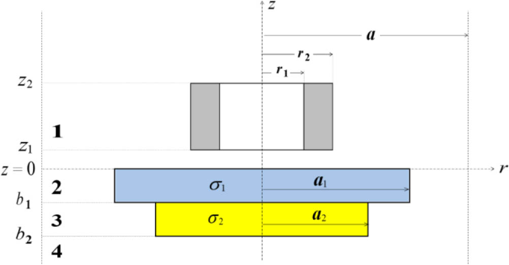 (5) U=∫0arF1(r)F2(r)dr==R1(p1a1)R1(p2a2)∫0a2rJ1(q1r)J1(q2r)dr++R1(p1a1)J1(q2a2)∫a2a1rJ1(q1r)R1(p2r)dr++J1(q1a1)J1(q2a2)∫a1arR1(p1r)R1p2rdr. \matrix{{{\boldsymbol{U}} = \int_0^a {r{{\boldsymbol{F}}_1}(r){{\boldsymbol{F}}_2}(r){\rm{d}}r =}} \cr {= {{\boldsymbol{R}}_1}({{\boldsymbol{p}}_1}{a_1}){{\boldsymbol{R}}_1}({{\boldsymbol{p}}_2}{a_2})\int_0^{{a_2}} {r{{\boldsymbol{J}}_1}({{\boldsymbol{q}}_1}r){{\boldsymbol{J}}_1}({{\boldsymbol{q}}_2}r){\rm{d}}r +}} \cr {+ {{\boldsymbol{R}}_1}({{\boldsymbol{p}}_1}{a_1}){{\boldsymbol{J}}_1}({{\boldsymbol{q}}_2}{a_2})\int_{{a_2}}^{{a_1}} {r{{\boldsymbol{J}}_1}({{\boldsymbol{q}}_1}r){{\boldsymbol{R}}_1}({{\boldsymbol{p}}_2}r){\rm{d}}r +}} \cr {+ {{\boldsymbol{J}}_1}({{\boldsymbol{q}}_1}{a_1}){{\boldsymbol{J}}_1}({{\boldsymbol{q}}_2}{a_2})\int_{{a_1}}^a {r{{\boldsymbol{R}}_1}({{\boldsymbol{p}}_1}r){{\boldsymbol{R}}_1}\left({{{\boldsymbol{p}}_2}r} \right){\rm{d}}r.}} \cr}

Fig. 1.

Cross-section of a coil located over a disc with two layers of different diameters.

Afterwards, using the formulas for the expansion of the integrals of products of special functions, the subsequent terms of the matrix U were written as sums of series. (6) uik=a2R1(p1,ia1)R1(p2,ka2)q1,i2−q2,k2[q2,kJ1(q1,ia2)J0(q2,ka2)−q1,iJ0(q1,ia2)J1(q2,ka2)++R1(p1,ia1)J1(q2,ka2)q1,i2−p2,k2{a1[p2,kJ1(q1,ia2)R0(p2,ka1)−q1,iJ0(q1,ia1)R1(p2,ka1)]−−a2[p2,kJ1(q1,ia2)R0(p2,ka2)−q1,iJ0(q1,ia2)R1(p2,ka2)]}−−J1(q1,ia1)J1(q2,ka2)p1,i2−p2,k2a1[p2,kR1(p1,ia1)R0(p2,ka1)−p1,iR0(p1,ia1)R1(p2,ka1)] \matrix{{{u_{ik}}} \hfill & {= {{{a_2}{{\boldsymbol{R}}_1}({{\boldsymbol{p}}_{1,i}}{a_1}){{\boldsymbol{R}}_1}({{\boldsymbol{p}}_{2,k}}{a_2})} \over {{\boldsymbol{q}}_{1,i}^2 - {\boldsymbol{q}}_{2,k}^2}}[{{\boldsymbol{q}}_{2,k}}{{\boldsymbol{J}}_1}({{\boldsymbol{q}}_{1,i}}{a_2}){{\boldsymbol{J}}_0}({{\boldsymbol{q}}_{2,k}}{a_2}) - {{\boldsymbol{q}}_{1,i}}{{\boldsymbol{J}}_0}({{\boldsymbol{q}}_{1,i}}{a_2}){{\boldsymbol{J}}_1}({{\boldsymbol{q}}_{2,k}}{a_2}) +} \hfill \cr {} \hfill & {+ {{{{\boldsymbol{R}}_1}({{\boldsymbol{p}}_{1,i}}{a_1}){{\boldsymbol{J}}_1}({{\boldsymbol{q}}_{2,k}}{a_2})} \over {{\boldsymbol{q}}_{1,i}^2 - {\boldsymbol{p}}_{2,k}^2}}\{{a_1}[{{\boldsymbol{p}}_{2,k}}{{\boldsymbol{J}}_1}({{\boldsymbol{q}}_{1,i}}{a_2}){{\boldsymbol{R}}_0}({{\boldsymbol{p}}_{2,k}}{a_1}) - {{\boldsymbol{q}}_{1,i}}{{\boldsymbol{J}}_0}({{\boldsymbol{q}}_{1,i}}{a_1}){{\boldsymbol{R}}_1}({{\boldsymbol{p}}_{2,k}}{a_1})] -} \hfill \cr {} \hfill & {\,\,\,\,\,\,\,\,\,\,\,\,\,\,\,\,\,\,\,\,\,\,\,\,\,\,\,\,\,\,\,\,\,\,\,\,\,\,\,\,\,\,\, - {a_2}[{{\boldsymbol{p}}_{2,k}}{{\boldsymbol{J}}_1}({{\boldsymbol{q}}_{1,i}}{a_2}){{\boldsymbol{R}}_0}({{\boldsymbol{p}}_{2,k}}{a_2}) - {{\boldsymbol{q}}_{1,i}}{{\boldsymbol{J}}_0}({{\boldsymbol{q}}_{1,i}}{a_2}){{\boldsymbol{R}}_1}({{\boldsymbol{p}}_{2,k}}{a_2})]\} -} \hfill \cr {} \hfill & {- {{{{\boldsymbol{J}}_1}({{\boldsymbol{q}}_{1,i}}{a_1}){{\boldsymbol{J}}_1}({{\boldsymbol{q}}_{2,k}}{a_2})} \over {{\boldsymbol{p}}_{1,i}^2 - {\boldsymbol{p}}_{2,k}^2}}{a_1}[{{\boldsymbol{p}}_{2,k}}{{\boldsymbol{R}}_1}({{\boldsymbol{p}}_{1,i}}{a_1}){{\boldsymbol{R}}_0}({{\boldsymbol{p}}_{2,k}}{a_1}) - {{\boldsymbol{p}}_{1,i}}{{\boldsymbol{R}}_0}({{\boldsymbol{p}}_{1,i}}{a_1}){{\boldsymbol{R}}_1}({{\boldsymbol{p}}_{2,k}}{a_1})]} \hfill \cr}

A general expression for the change in the impedance of a coil over conductive material was formulated in [5] as: (7) ΔZ=jω2πN2(r2−r1)2(z2−z1)2∫z1z2∫r1r2rA1(r,z)drdz. \Delta Z = {{j\omega 2\pi {N^2}} \over {{{({r_2} - {r_1})}^2}{{({z_2} - {z_1})}^2}}}\int_{{z_1}}^{{z_2}} {\int_{{r_1}}^{{r_2}} {r{A_1}(r,z){\rm{d}}r\,{\rm{d}}z}}. where ω is the angular frequency of the probe, A₁ is the magnetic potential of region 1, and N is the number of coil turns. After determining the elements of the U matrix and integrating over the coil volume, the final formula for a probe placed above a double-layer disc was derived (Fig. 1). (8) ΔZ=jω2πN2(r2−r1)2(z2−z1)2∑j=1∞κ(αj)e−αjz2−e−αjz1αjD1,j \Delta Z = {{j\omega 2\pi {N^2}} \over {{{({r_2} - {r_1})}^2}{{({z_2} - {z_1})}^2}}}\sum\limits_{j = 1}^\infty {\kappa ({\alpha _j}){{{e^{- {\alpha _j}{z_2}}} - {e^{- {\alpha _j}{z_1}}}} \over {{\alpha _j}}}{D_{1,j}}} and the coefficient D_1,j is defined in [15].

Equation (7) was implemented in Matlab. The calculations were performed for 75 frequency values ranging from f=500 Hz to f = 15 kHz. The air-core probe was then connected to the Keysight E4980A precision LCR meter using Kelvin clips. The probe used, with a height of z₂−z₁=5 mm and a radial width of r₂−r₁=2.8 mm, had 1550 turns. Two sets of discs made of different materials, with the parameters presented in Table 1, were prepared. The first step consisted of measuring the impedance Z₀=R₀+jX₀ for the probe placed at a distance from the conductive material. Subsequently, impedance Z=R+jX was measured after the probe was placed on the double-layer disc. The normalised values of the changes in resistance (R−R₀)/X₀, obtained from the measurements and calculations, are presented in Fig. 2, and the normalised values of the changes in reactance (X−X₀)/X₀ are shown in Fig. 3. In all of the cases, the difference in the values of the probe impedance components obtained from the calculations and measurements did not exceed 2 %. The results of the measurements and calculations were also compared for two frequency values in Table 2. The error was slightly smaller for changes in resistance ΔR=R−R₀ than for changes in reactance ΔX=X−X₀.

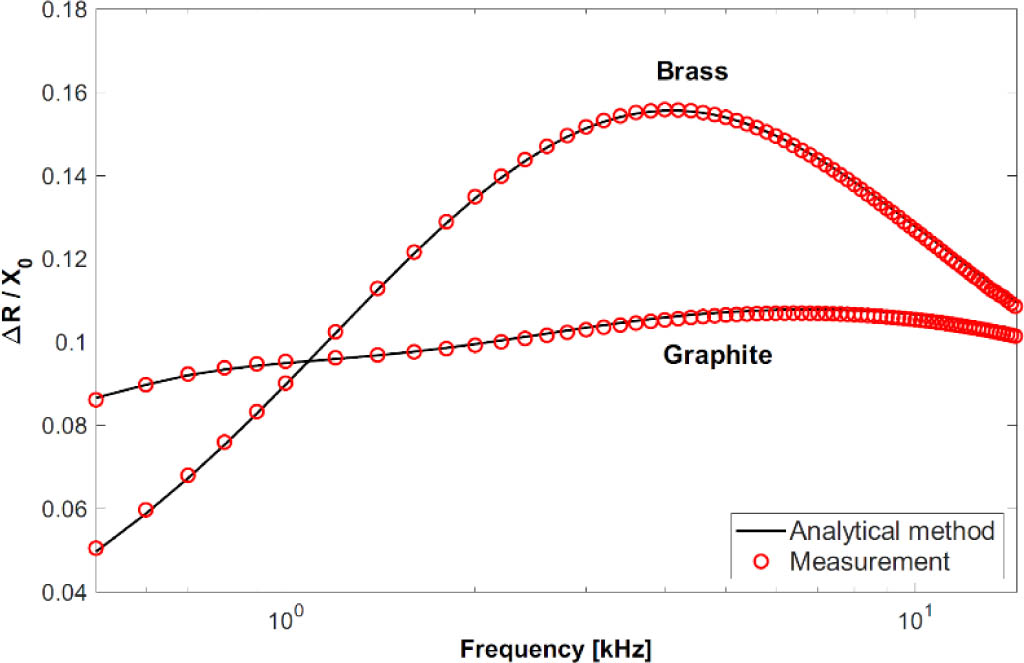
Fig. 2.

Normalised changes in the resistance ΔR.

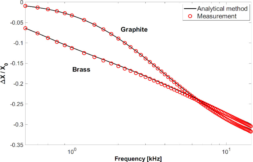
Fig. 3.

Normalised changes in the resistance ΔX.

The proposed analytical model enables calculation of changes in the probe impedance when it is placed over a conductive disc, with the upper layer having a larger diameter than the lower layer. The disc layers may have any thickness, diameter, and electrical conductivity. The final formula for the change in probe impedance was written in closed form to be implemented in any computational package or programming language. The calculation results for the two disc configurations showed a small error, which did not exceed 2 %. Therefore, the developed model can be successfully employed for computer simulations of eddy current inspections of elements, such as screws, rivets, and valves. Further work is planned to develop analytical solutions for probes containing coils with a core and for other shapes of tested components.