
1. INTRODUCTION
Machine learning (ML) has become a transformative technology in the medical field, particularly in disease prediction. By inspecting enormous amounts of data and recognizing patterns that might be imperceptible to the human eye, ML based algorithms can appreciably enhance the precision and effectiveness of disease prediction [1]. This capability is crucial for timely diagnosis, personalized care and improved patient outcomes [2]. Deep learning (DL), a subcategory of ML, has made significant progress across diverse sectors, particularly in healthcare. DL’s capability to handle and transform an enormous quantity of multifaceted data has placed it in the most preferred position for disease prediction and diagnosis. By leveraging deep neural networks, DL models can uncover complicated patterns and associations embedded in medical corpora, leading to improved accuracy and early disease detection [3]. The most predominant use of DL models in disease prediction is in the analysis of medical images. Convolutional neural network (CNN) excel at processing pixel data in images, making them ideal for detecting abnormalities in X-rays, MRIs, and CT scans [4]–[6].
DL in disease prediction involves training algorithms on historical patient records to identify patterns and correlation that indicate the presence or likelihood of a disease. The predictive models developed through this process can analyze new patient data to forecast potential health issues. This approach can be applied to diversified diseases, such as cancer, cardiovascular diseases, diabetes, and infectious diseases [7]. DL has the potential to drive significant advancements across various fields, but it also faces numerous challenges that must be addressed to realize its full potential. Issues related to data requirements, computational resources, model interpretability, generalization, ethical considerations, robustness, and research reproducibility present significant obstacles. Hyperparameters are significant for training and improving the efficiency of DL models. In traditional models, the parameters used to generate models are initialized and subsequently updated iteratively through the training process. When inappropriate parameter values are initialized, the performance of DL models will be reduced abruptly, as these parameters control various aspects of the model’s architecture and training process. Selecting and tuning hyperparameters is a critical and often challenging task, as it significantly influences the effectiveness and efficiency of DL models. This paper explores the key issues associated with hyperparameters in DL and key methodologies for hyperparameter tuning [8]–[9].
Hyperparameters influence the effectiveness of DL models in disease prediction. Effective tuning of these parameters is essential to develop robust, accurate, and efficient predictive models. While challenges such as high dimensionality, computational cost, data scarcity, and the need for interpretability exist, advanced tuning techniques and thoughtful strategies can address these issues. We propose a hyperparameter optimization technique that enhances disease prediction models to improve healthcare outcomes through early and accurate diagnosis [10].
Pneumonia is an acute inflammatory disease that affects the alveoli present in the lungs. Accurate and timely diagnosis is critical for effective treatment and decreasing mortality rates. Conventional methods of pneumonia diagnosis rely on clinical trials and imaging techniques such as chest X-ray (CXR), interpreted by radiologists. However, interpreting X-rays can be subjective and time-consuming. DL, particularly CNNs, offers a promising approach to automate and improve the accuracy of classifying pneumonia from CXR images [11].
A news report promulgated on World Pneumonia Day estimates that pneumonia could cause the deaths of over 11 million children under the age of five by 2030 [12]. In the early 19th century, pneumonia was a leading cause of death. Historically, doctors used clinical examinations, medical histories, and CXR to identify pneumonia. Today, technological advancements have made CXR more affordable, and it is widely used to detect pneumococcal diseases [13]. The shortage of medical experts can be mitigated by employing various computerized methodologies. Advances in artificial intelligence (AI) have been beneficial for disease diagnosis; for example, CNNs are used to classify CXR for pneumonia detection. Research in abnormal pattern detection, biometric recognition, trauma severity assessment, airport accident prevention, efficiency prediction using artificial neural networks (ANN), and bone pathology diagnosis [14] has shown promising results. However, the high variability in image features affects retrieval accuracy.
CNNs have adopted image analysis by automatically extracting significant features hierarchically from image pixel data. CNNs comprise several layers, such as convolutional layers, pooling layers, and fully connected layers, that progressively extract highly complex, multifaceted image features. This capability makes CNNs well-suited for medical image analysis tasks, such as detecting pneumonia from CXR [15]. Many researchers explored the detection of pneumonia utilizing DL methodologies. Their investigation delves into the use of DL techniques for detecting pneumonia from chest radiograph images. Their study aims to assess the efficacy of DL techniques in recognizing pneumonia from medical imaging datasets [16]–[18].
An explainable ML model was used to categorize diseases relevant to chest infections, namely pneumonia, Covid-19, and lung cancer. Their research primarily focuses on decipherable ML models for categorizing pneumonia, tuberculosis, and Covid-19 from CXR images. Their methodology extracts features from CXR images based on texture and enhances categorization accuracy.
The use of Progressive Web Applications for the deployment of ML models to predict mortality in children born in Gambia using a neural network model was reported [19]. A computerized tool was designed to identify lung related diseases from CXR images [20]. Their study focuses mainly on improving the accuracy and effective categorization of the above-mentioned diseases at minimal cost.
2. Proposed Pneumonia Detection and Hyperparameter Optimization Model
While designing ML models, optimization techniques for exploring the hyperparameter space can pinpoint the best hyperparameter settings. This optimization process involves four key components: an estimator with its objective function, a search space, a search or optimization method, and an evaluation function. The estimator might be a classifier or regressor for which the model parameters need to be optimized. The search space, also known as configuration space, contains all possible parameter values. An optimization method discovers optimal hyperparameter combinations for the estimator. An evaluation function assesses the efficiency of various configurations of hyperparameters.
In practical applications, continuous and discrete hyperparameters often have bounded domains [21]. Moreover, the configuration space for hyperparameters may involve conditional relationships. A hyperparameter might require adjustment based on another hyperparameter value, referred to as a conditional hyperparameter. In support vector machines, the kernel function degree is significant only when a polynomial-based kernel is used.
The hyperparameter’s values can be represented as an n-dimensional real-valued vector space. The hyperparameters also frequently presume diverse domain values with varying constraints. Hence, the problem of hyperparameter optimization becomes an intricate constrained optimization problem. For example, the quantity of features considered in a decision tree ought to fall within the spectrum from 0 to n, where n is the number of training features, whereas in k-means clustering, the maximum clusters must not exceed the data point size [22]. Furthermore, features that are categorical in nature often have limited options, such as the choice of activation function or neural network optimizer. Hence, the feasible subset of parameter values commonly has a highly complex, multifaceted configuration, thereby increasing the intricacy of the problems at hand [23].
The goal of HPO is to achieve the best possible or near-best performance from a model by adjusting hyperparameters within specified constraints. This can be expressed as function f that may be varied based on the chosen DL model’s objective function and the evaluation metric. Models can be assessed using a range of metrics, such as RMSE, accuracy, F1-Score, and false alarm rate. Conversely, time constraints are a crucial consideration in hyperparameter optimization (HPO) in real-world scenarios. Achieving optimal results often demands significant time investment because it requires testing numerous hyperparameter configurations. Each test of a hyperparameter requires retraining the entire ML model and processing the validation set to generate a performance score [24].
The primary procedure of HPO unfolds as follows:
Choosing the appropriate objective function and evaluation metrics.
Identifying hyperparameters for tuning, categorizing, and selecting an appropriate optimization technique.
Training DL models with preset hyperparameter values as the reference.
Optimizing the hyperparameter values by manual experimentation and domain expertise.
Updating the search space with the best hyperparameter values obtained. If needed, use a new search space.
Concluding by selecting the configuration that yields the best performance as the ultimate solution.
However, the majority of conventional optimization methods are not well-suited for HPO due to distinct disparities between HPO problems and conventional optimization challenges. These disparities manifest in several key aspects and research gaps as follows:
The objective functions of DL models are generally non-convex and non-differentiable. Consequently, numerous traditional techniques tailored for convex or differentiable problems may lead to local optima rather than global optima in HPO scenarios. Moreover, the lack of smoothness in the optimization target renders certain conventional derivative-free optimization models ineffective for the challenges posed.
DL model hyperparameters encompass a variety of types, including conditional, categorical, discrete, and continuous parameters. Consequently, many traditional optimization approaches focus solely on numeric continuous variables and are inadequate for addressing the complexity of HPO problems.
Training ML models on large-scale datasets often incurs significant computational expenses. To mitigate this, HPO techniques modify the objective function using data sampling. Hence, an effective HPO should be able to leverage these modifications.
Main ideas, theory, and mathematical formulations should be provided, along with data on the measurement method and instruments as well as experimental results. This part should be accompanied by specific references.
A. Existing optimization algorithms
Grid search optimization (GSO) is as the most straightforward approach to fine-tuning hyperparameters. Essentially, it involves partitioning the hyperparameter space into a discrete grid, systematically testing each grid point’s combination through cross-validation to evaluate performance metrics. The highest average grid point emerges as the set of optimal hyperparameters. While grid search exhaustively explores all possible arrangements, ensuring the discovery of the best solution within the domain, its major drawback is its time-consuming nature. The exhaustive search across the entire parameter space demands considerable computational resources, making it impractical in time-sensitive scenarios. Moreover, each grid point necessitates K-fold cross-validation, amplifying the complexity and cost of hyperparameter tuning. Nonetheless, for those seeking the most optimal hyperparameter configuration, grid search remains a compelling choice. In GridSearchCV, cross-validation is seamlessly integrated with grid search, further enhancing the model training process [25]. Cross-validation ensures robust model evaluation prior to deployment [26].
Random search optimization (RSO) resembles grid search; however, instead of employing all grid points, it evaluates only a randomly selected subset of these points. The smaller this subset, the quicker but less precise the optimization becomes. Conversely, with a larger subset, the optimization accuracy increases, but it begins to resemble a grid search more closely. This approach proves highly beneficial when confronted with numerous hyperparameters featuring a finely divided grid of values. By selecting a random subset of 5 to 100 points, we can obtain a reasonably satisfactory set of hyperparameter values. While it may not yield the optimal solution, it can still provide a commendable set of values leading to a well-performing model [27].
A more attractive strategy for automatically refining hyperparameters is through the Bayesian optimization (BO) algorithm. It is characterized by its informed search nature, which ensures that each iteration learns from the preceding one, with the outcomes of each iteration guiding the creation of the next. Sampling a subset of hyperparameter combinations is the same in both BO and RSO, yet their selection methods differ [28]. In BO, the tuning process is conceptualized as the optimization of a black box function that optimizes the model’s final prediction score. A surrogate model is used to minimize the objective function [29]. While various surrogate models exist for BO, the most prevalent is the Gaussian model. Initially, a random subset of hyperparameter combinations is selected and evaluated. The objective function is then constructed using the above chosen random subset. Further, two methods are used to select the next set of values, opting for a value near the highest attained value or exploring another subset of the search space.
BO functions are expressed by a posterior distribution of functions. When the data corpus scales to enormous proportions, it refines, thereby enhancing the model’s confidence in identifying worthwhile and unworthy regions within the parameter space. Through successive iterations, the model maintains a balance between exploration and exploitation, leveraging its understanding of the target function. At each iteration, a Gaussian process is adjusted to incorporate the known samples (previously explored points), and the posterior distribution, coupled with an exploration strategy, guides the selection of the next exploration point.
Particle swarm optimization (PSO) is a community based optimization strategy that mimics the collective behavior of birds and animals. PSO is employed to solve various types of problems in an optimal way by iteratively improving candidate solutions with respect to a given measure of quality.
A set of particles constitutes a swarm. Each particle represents a candidate solution that has a position in solution space and a velocity that determines the particle’s movement through the solution space. The optimality of a particular solution is assessed using a fitness function. The goal is to maximize (or minimize) this fitness function. The particle’s position and velocity are updated based on its past activities and the activities of surrounding particles in the swarm [30]. Equation (1) is used to determine the velocity of the particle:
where Vi(t) is the ith particle velocity at instant t, ω is the weight when the particle is in idle state, c1 denotes the particle’s best position and c2 represents the swarm’s best position. r1 and r2 are real numbers generated randomly that range between 0 and 1, pbesti is the paramount position identified by the individual particle, and gbesti is the paramount position identified by the swarm. Based on the present position xi(t), the position of the particle is updated using (2):B. Elephant herd optimization (EHO)
Elephants, being social creatures, inhabit matriarchal communities alongside females and their young. A group of elephants, known as a clan, consists of multiple individuals and is guided by a matriarch. Females typically opt to stay close to their relatives, whereas male leaders tend to roam independently, gradually establishing full autonomy from their familial ties [31].
The size of each elephant clan is limited. The male elephants from the clan leave their family and live independently in a distant area. A matriarch presides over the elephants in each clan. According to elephant behavior, each clan is led by a matriarch who oversees the elephants. Consequently, the matriarch determines each elephant’s new position. Equation (3) illustrates how to calculate an elephant’s position within the clan.
The PCn,m represents the elephant position m in a clan Cn before the departure of the male elephant, whereas Pnew,Cn,m represents the positions of the elephant after the departure. The clan matriarch, denoted as Pbest,Cn, is the best and fittest elephant. The new position s is a scale factor that lies in the range [0, 1] and influences the matriarch, while f represents the paramount position of the elephant and lies within the range [0, 1].
The optimal elephant in the clan is determined by (4), where ω in the range [0, 1] affects the new position of the elephants at Pcenter,Cn and the influence of Cn on the best-fit elephant Pnew,Cn,m.
The central individual of the clan is Pcenter, calculated using (5).
Here, 1 ≤ z ≤ Z and GCn denote the population of elephants in clan Cn, and PCn,z represents the position of individual elephant PCn,m,z in the z dimension. Therefore, Pcenter,Cn,z is the new paramount position of an elephant in clan Cn, revised through (5).
In addressing optimization problems, the separation operator models the process by which male elephants leave their community. As shown in (6), the elephant having poor performance within the community in each generation uses the separation operator.
Here, Pmax and Pmin represents the upper and lower limit for each elephant’s position in the community. Pworst,Cn refers to the inferior elephant of clan Cn. Rand[0,1] is a random variable whose values lie between 0 and 1.
C. Adaptive EHO using Python rectilinear locomotion strategy (AEHO-PRLS)
Snakes possess flexible, elongated bodies that allow them to navigate all sorts of terrains, like tree trunks, narrow crevices, foliage, or sand, with ease. In tight spaces, they employ a rectilinear locomotion movement mechanism to move forward, similar to the movement of earthworms. Rectilinear locomotion is a mechanism of movement in which an organism moves in a straight line, typically used by creatures such as snakes. In the context of optimization problems, rectilinear locomotion techniques can be applied in various ways to explore the solution space and converge towards the best possible solutions, which are more optimal. In rectilinear locomotion, movement is constrained to straight lines. Similarly, in optimization problems, search algorithms can be designed to explore solutions along straight paths in the solution space. This can be done by iteratively adjusting one variable at a time while keeping others constant, following a straight-line trajectory through the multidimensional space [32].
Rectilinear paths can be associated with grid-based searches in which the solution space is discretized into a grid, and movements are restricted to grid lines. This is mainly useful for domain problems whose search space can be naturally divided into discrete steps.
Rectilinear movement concepts can be integrated into simulated annealing by restricting the neighborhood exploration to rectilinear paths. By adapting rectilinear locomotion principles, optimization algorithms can efficiently navigate constrained spaces, yielding practical and efficient solutions across domains such as engineering, logistics, and computational biology [33].
The snakes are represented as 1D linked list n-linked crawlers. The n-linked crawlers are generated using a model similar to the concertina locomotion mechanism. First, nodes representing crawlers are connected by extensible muscles via a series of k − 1 inter-nodal elements, and changes in length describe the snake motion, simulating tiny wave-like movements. The model accepts the snake’s wave-like movement by modeling wave kinematics with friction coefficients as inputs and produces the position of the snake at the center of mass, m, as output. For each node that lies on the surface, the friction force Fi is determined using the sliding friction law and is mathematically expressed as in (7)
Here, FN represents the normal force owing to the weight of the node, while mi indicates the speed of the node. The frictional coefficients μi for the ventral surface after applying the sliding frictional law are constituted by two coefficients μf and μb, where μf is the coefficient when the movement is in the forward direction and μb is the coefficient when the movement is in the reverse direction. At each node, Newton’s second law is applied, taking into account both inter-node forces and friction. The equation that governs the movement of n-linked crawlers with the snake’s center of mass m is given in (8):
where is the Heaviside function [32] used to calculate the step, the inclination angle is θ, and the Froude number [33] is represented by (9):The movement of n-linked crawlers is modeled by body length L, contraction and extension period τ, and gravitational acceleration g. The very low Froude number indicates that the force due to inertia is much smaller than the force of gravity. Froude numbers Fr ≈ 0.002 to 0.006 have 1 or 2 orders of magnitude higher inertial forces. Froude number Fr ≈ 0.02 represents slithering motion. Obviously, the crawler movement involving rectilinear locomotion has lower inertia.
Combining rectilinear locomotion techniques with EHO can create an innovative hybrid optimization algorithm that leverages the power of both approaches. EHO, a swarm intelligence-based algorithm, is motivated by the social behavior and migration patterns of elephant herds. Incorporating rectilinear locomotion into EHO can help refine the model’s exploration and exploitation phases, potentially enhancing its performance.
To integrate rectilinear locomotion, we can modify the movement update rules within the EHO framework to include straight-line exploration. This involves constraining the movement of elephants along coordinate axes, which can help systematically explore the search space.
By combining rectilinear locomotion with EHO, the algorithm can benefit from systematic exploration along coordinate axes while maintaining the global search capabilities of swarm intelligence. This hybrid approach, as described in the table, can potentially improve convergence speed and solution quality for various optimization problems. The architecture of the proposed system is denoted in Table 1.
3. Experimental Results
The results of the AEHO-PRLS model and its comparison with existing models are discussed in this section. Fig. 1(a) represents clear lungs from a normal chest X-ray. Fig. 1(b) depicts pneumonia caused by a virus, having an interstitial lung pattern, and Fig. 1(c) represents pneumonia caused by bacteria, showing focal lobar consolidation.
Table 2.
Distribution of the dataset.
| No. of images | Class |
|---|---|
| 1281 | Covid-19 CXRs |
| 3270 | Normal CXRs |
| 1656 | Viral pneumonia CXRs |
| 3001 | Bacterial pneumonia CXRs |
The combined dataset is obtained from Mendeley [34] and Kaggle [35], comprising 9208 CXR images. The dataset is divided into 3 directories, namely train, test, and val, with sub-directories for each classification of the image as mentioned in Table 2. Different CNN models are generated by applying different hyperparameter tuning mechanisms, such as GSO, RSO, BO, PSO, EHO, and AEHO-PRLS. The train-test split considered for the study is 70 % for training, 15 % for testing, and 15 % for validation. The values of the hyperparameter chosen by different optimization algorithms are shown in Table 3. After training a model, performing a thorough analysis is essential to understand its performance, identify potential issues, and determine areas for improvement. The following metrics are used to assess and compare the efficiency of the CNN model across various hyperparameter values determined by a variety of optimization strategies.
Algorithm
Step 1: Population initialization
➢ The hyperparameters are the elephants. Initialize the elephant population for each clan and the number of clans.
Step 2: Formulate fitness function
➢ In order to obtain the best solution, a fitness function fn is assessed for all the agents in the search space and the agent with minimal fitness value is chosen as the paramount search agent Pbest,Cn.
where Ci is the ith centroid,fj are data points corresponding to ith centroid,
D and W represent the dimension values.
Step 3: Revise the search agent’s position
➢ Search agent’s position is revised.
Step 3a: Clan update operator
where Pnew,Cn,m is the new position for elephant m in clan n,PCn,m is the old position for elephant m in clan n,
∝ ∈ (0,1) is the uniform random distribution,
x = 1 − t/T,
t is the current iteration,
T is the maximum number of iterations,
Pbest,Cn is the near-optimal elephant in clan Cn.
Step 3b: Position update
Update the position of the near-optimal elephant using the python rectilinear locomotion strategy
(i) Compute adaptive parameter d using the python rectilinear locomotion strategy
where μa and μb are sliding frictional coefficients of the ventral surface,n is the number of nodes in the search surface,
is the Heaviside step function and
the angle of inclination is θ.
(ii) Update the position of the fittest elephant
where d is the adaptive parameter computed using the previous step, where 1 ≤ m ≤ M represents the m dimension and M represents the total dimension.
Step 4: Remove outlier
➢ Remove the outlier points in the search space using the clan separating operator
where Pmax and Pmin are the upper limit and lower limit for elephant position,Rand ∈ (0,1) is the uniform random distribution.
Step 5: Evaluate feasibility
➢ Search agent’s fitness is assessed using Step 2, and the fittest search agent is considered as the optimal solution.
Step 6: Termination
➢ The steps 1 to 5 are iterated until the best solution converges as optimal.
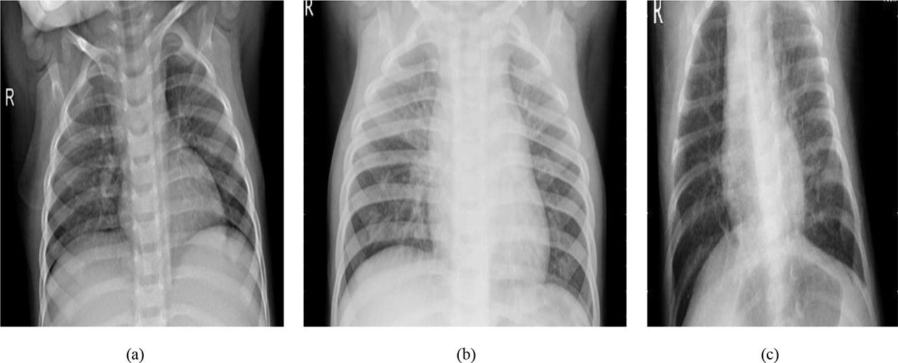
Fig. 1.
Sample images from dataset.
Table 3.
Hyperparameter values against various optimization algorithms.
| Model | Dropout_1 | Filter count | Dropout_2 | Dense_activation | Dropout_3 | Learning rate | Units | Epochs | Score | Loss | Accuracy |
|---|---|---|---|---|---|---|---|---|---|---|---|
| GSO | 0.2 | 32 | 0.3 | softmax | 0.1 | 0.0059 | 32 | 25 | 0.1006 | 0.8929 | 0.7357 |
| RSO | 0.35 | 64 | 0.45 | softmax | 0.1 | 0.0052 | 192 | 45 | 0.1408 | 0.7412 | 0.7659 |
| BO | 0.05 | 256 | 0 | softmax | 0.15 | 0.002419 | 448 | 15 | 0.1789 | 0.4893 | 0.7492 |
| PSO | 0.25 | 128 | 0.25 | softmax | 0.07 | 0.00171507 | 260 | 40 | 0.2121 | 0.4893 | 0.8931 |
| EHO | 0.2 | 128 | 0.1 | softmax | 0.05 | 0.0038287 | 256 | 35 | 0.6556 | 0.296 | 0.9237 |
| Proposed AEHO-PRLS | 0.1 | 64 | 0.05 | softmax | 0.01 | 0.00024914 | 256 | 28 | 0.727 | 0.1586 | 0.9657 |
Accuracy: The proportion of correctly classified instances as given by (10).
Precision: As mentioned in (11), precision is the ratio of true positive instances and all positive predictions.
Recall: Recall is the ratio of true positives and all real positives as given by (12).
Specificity: Specificity is represented in (13) as the measure of the true negative rate.
F1-Score: F1-Score is represented in (14) as the harmonic mean of precision and recall.
The efficiency of the proposed AEHO-PRLS model was measured using a test set after the training phase. The accuracy of the proposed AEHO-PRLS model was 96.57 %. The precision was 96.73 %, indicating the ability of the model to classify true positives accurately.
This is vital in circumstances where false positives have a serious negative impact. The proposed model has an F1-Score of 94.18 %, indicating an equilibrium between precision and recall. Also, the model achieved AUC of 0.9564 and 95.51 % specificity, reflecting its ability to accurately distinguish between classes and its resilience against false positives. Fig. 2 presents the performance of the baseline models, their variants, and the proposed AEHO-PRLS model on various evaluation metrics. The proposed AEHO-PRLS model exhibits better efficiency than the other models.
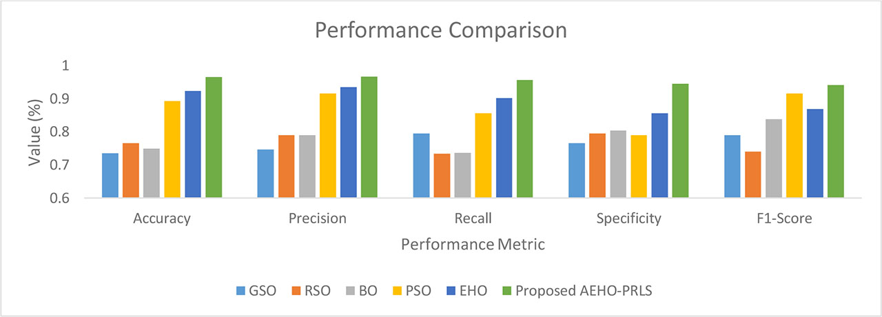
Fig. 2.
Performance comparison of the proposed model.
A. Statistical analysis
A paired t-test was conducted between the proposed AEHO-PRLS model and baseline optimization methods to ensure the statistical reliability of the results. It was conducted across multiple experimental runs for accounting variable training with a null hypothesis assumption regarding the difference in performance of the models. The obtained p-values are less than 0.05, indicating that the proposed model is statistically significant at the 95 % confidence level. The results also ensure that the performance gains are driven by the effective optimization model rather than random variations.
B. Ablation study
The ablation study was conducted to evaluate the individual contributions of the components in the proposed framework. The evaluation consisted of baseline CNN, CNN with EHO, and PRLS individually, and finally, CNN combined with the AEHO-PRLS model. The results of the study are listed in Table 4.
C. Comparative analysis
A comparative study with ResNet50, DenseNet121, and EfficientNet80 was performed to further evaluate the proposed model. These models are considered strong baselines in medical image classification tasks, owing to their deep architecture and transfer learning capabilities. The results in Table 5 indicate that the proposed model improves the classification accuracy compared to the baseline models. This also necessitates the use of effective optimization techniques to improve DL models for medical imaging applications.
Table 5.
Comparative analysis.
| Model | Accuracy [%] |
|---|---|
| ResNet50 | 92.9 |
| DenseNet121 | 93.6 |
| EfficientNetB0 | 94.01 |
| Proposed AEHO-PRLS | 96.57 |
To evaluate classification effectiveness, a comparative analysis with widely used hyperparameter optimization techniques was conducted, and the results are shown in Table 6. The proposed AEHO-PRLS model achieves approximately 7.37 % improvement over EHO and 26.17 % improvement over GSO, thereby demonstrating a superior optimization capability. The consistent improvement across all evaluation metrics indicates the robustness and reliability of the proposed framework.
Table 6.
Performance comparison.
| Model | Accuracy | Precision | Recall | F1-Score |
|---|---|---|---|---|
| GSO | 73.57 | 74.96 | 76.57 | 74.62 |
| RSO | 76.59 | 73.82 | 72.58 | 73.10 |
| BO | 74.92 | 76.14 | 79.24 | 73.51 |
| PSO | 89.31 | 84.21 | 83.64 | 83.94 |
| EHO | 92.37 | 90.21 | 90.97 | 89.75 |
| Proposed AEHO-PRLS | 96.57 | 95.73 | 94.02 | 94.23 |
The proposed model also demonstrates stable performance across multiple runs, indicating strong generalization capability. The computational complexity of the proposed model is governed by population size (N), iteration count (T), and dimensionality of the hyperparameter space (D), as represented in (15).
The proposed model slightly increases the computational overhead compared to EHO. This is compensated for by faster convergence and improved solution quality, thereby minimizing the iteration count needed for optimal performance.
4. Novelty
The proposed AEHO-PRLS framework introduces a structured search mechanism into the traditional EHO, which primarily focuses on global exploration along clan-based updates. EHO is inefficient in local exploitation, leading to premature convergence. The integration of PRLS removes the limitation of axis-aligned deterministic search, improving convergence precision and stability. Key novelties of the proposed research work are listed below:
Hybridization of swarm intelligence with deterministic rectilinear search.
Improved exploration-exploitation balance.
Faster convergence in high-dimensional hyperparameter space.
5. Conclusion
This paper explores the critical role of hyperparameter optimization in improving the efficiency of DL models for the identification of pneumonia in CXR images. By exploring various baseline optimization techniques such as GSO, RSO, BO, PSO, EHO, and AEHO-PRLS, the significant impact of effective hyperparameter tuning on model accuracy and efficiency is demonstrated. The proposed AEHO-PRLS achieved superior performance, with 96.57 % accuracy, 96.73 % precision, and 94.18 % F1-Score. These metrics indicate an unbiased performance among precision and recall, highlighting the robustness of the AEHO-PRLS model in handling the complexities of medical image analysis. The AEHO-PRLS model’s ability to enhance disease prediction models is particularly significant for pneumonia, a major global health challenge that affects millions each year.
The integration of advanced optimization techniques into DL frameworks, as demonstrated in this paper, paves the way for more efficient and robust diagnostic tools in healthcare. Future work will focus on further refining the AEHO-PRLS model to enhance its generalizability and robustness. Additionally, exploring the applicability of this optimization strategy to other medical imaging tasks could broaden its impact and contribute to the development of comprehensive diagnostic systems. The promising results of this study encourage continued research and innovation in the field of medical image analysis, aiming to leverage technology for better healthcare outcomes.