
Conventional calibration procedures, while widely used, often face several limitations. These include insufficient monitoring of long-term stability, limited ability to detect systematic deviations, reliance on manual calculations that increase the risk of human error, and lack of integration with statistical process control (SPC) tools. Such drawbacks can reduce confidence in calibration results and hinder early detection of measurement drift.
To overcome these limitations, this study proposes a methodology that integrates SPC techniques (Shewhart charts) [1] with modern automation tools (Python-based monitoring and alarms). This combination enables real-time detection of deviations, enhances traceability to national standards, and strengthens the reliability of calibration outcomes.
The goal of this research is to develop and apply a robust quality assurance protocol for Pt-100 calibration at the National Institute for Standards (NIS), Egypt, combining SPC with automation to promptly detect deviations and improve measurement traceability.
To ensure the validity and reliability of calibration results, the thermal measurements laboratory at NIS applies a structured set of quality assurance practices. These include the use of reference materials and quality control (QC) samples to verify measurement accuracy, as well as employing alternative calibrated instruments to provide traceable results. Functional checks of measuring and testing equipment are routinely performed, and working standards are applied in conjunction with control charts to monitor stability.
Intermediate checks are conducted on measuring equipment to detect drift or malfunction, while replicate tests or calibrations using the same or different methods are carried out to assess repeatability. Retesting or recalibration of retained items is performed to confirm consistency over time, and correlation of results across different characteristics of the same item ensures coherence.
In addition, the laboratory has established an SPC-based procedure. Specifically, Shewhart charts (X̅, R, and S) and the capability index (Cp) are used to monitor calibration performance continuously. This integration of SPC provides a quantitative framework for detecting deviations and ensuring the long-term validity of calibration results.
Shewhart rules were based on acceptance criteria as:
- ≈
68.2 % of results lie between ±1σ (sample standard deviation).
- ≈
95.45 % of results lie between ±2σ.
- ≈
99.7 % of results lie between ±3σ.
These percentages are derived from the empirical rule of the normal distribution. However, it is important to note that SPC does not strictly require normal distribution. Control charts are robust tools that can be applied to processes with different distributions. The normal curve is often used for illustration because, according to the central limit theorem, subgroup means tend to approximate normality as sample size increases. In practice, SPC can be applied to non-normal data provided that appropriate chart types or transformations are used.
A control chart shows the state of control when: Two thirds of all points are near the center value. The points appear to float back and forth across the centerline.
The points are balanced on both sides of the centerline. No patterns or trends are observed.
The results are plotted on the vertical axis, and the date on the horizontal axis. For each calibration setting, 25 readings were collected (five groups of five repeated measurements). Collecting 25 readings instead of the initially planned 20 provided a stronger statistical basis. This adjustment improved the estimation of subgroup variability and enhanced the reliability of the control chart analysis, which serves as a model.
Steps for constructing the chart include:
Calculate the mean of the data series (X̅).
Calculate the standard deviation of the data series (s, sample standard deviation).
Calculate the upper and lower limits of the charts:
Upper control limit (UCL) UCL = Mean + 3StD = X + 3σ Upper warning limit (UWL) UWL = Mean + 2StD = X + 2σ Control line (CL) CL = Mean X Lower warning limit (LWL) LWL = Mean − 2StD = X − 2σ Lower control limit (LCL) CL = Mean − 3StD = X − 3σ Note: UWL and LWL are calculated using the mean
\mu \pm k\hat \sigma \hat \sigma \hat \sigma = \bar R/{d_2}
The Shewhart rules include the following conditions for detecting out-of-control situations:
One point outside 3σ control limits.
Two of three successive points outside 2σ on the same side.
Four of five successive points outside 1σ on the same side.
Eight successive points on the same side of the centerline.
Six consecutive points steadily increasing or decreasing.
Fourteen consecutive points alternating up and down.
Fifteen consecutive points within 1σ of the centerline.
Eight consecutive points outside 1σ but still inside 3σ.
A sudden change in mean level.
A systematic trend or cyclic pattern.
It is important to distinguish between Shewhart and Westgard rules. Shewhart rules are primarily applied in industrial and calibration contexts, where control charts are used to monitor process stability and detect out-of-control conditions. In contrast, Westgard rules are mainly applied in clinical laboratory settings, where they provide decision criteria for accepting or rejecting analytical runs of patient samples. While both sets of rules are based on statistical principles, their areas of application are distinct: Shewhart rules focus on process control, whereas Westgard rules focus on clinical quality control as shown in Table 1 [2], [3].
Distinction between Shewhart and Westgard rules in quality control.
| Aspect | Shewhart rules | Westgard rules |
|---|---|---|
| Origin | Walter A. Shewhart (industrial SPC) | James Westgard (clinical chemistry QC) |
| Application area | Manufacturing, engineering, calibration | Clinical laboratories, patient testing |
| Focus | Process stability & control | Analytical run validity & error detection |
| Tools used | X̅, R, S control charts | QC charts with multi-rule criteria |
| Decision outcome | Detects out-of-control process behavior | Accept/reject patient test runs |
The Westgard multi-rule QC procedure was initially developed for clinical laboratories to monitor the validity of patient test runs. In this study, the rules are adapted for calibration quality assurance. It is important to clarify that, in our context, the term “reject” does not mean discarding the resistance thermometer as inaccurate. Instead, it refers to rejecting the measurement series for that calibration run. When a rule is violated, the run is repeated or the equipment is inspected for possible sources of error. The instrument is only considered inaccurate if repeated runs consistently fail SPC criteria.
The most applied Westgard rules can be summarized as follows: [4]
Rule 1 (1–3s): A run is rejected if a single control measurement exceeds the mean ±3s. This is the classic out-of-control signal.
Rule 2 (2–2s): Two consecutive control measurements exceed the mean ±2s on the same side. In the original Westgard procedure this is a warning rule, that triggers closer inspection before applying rejection rules.
Rule 3 (R–4s): One control exceeds +2s and another exceeds −2s in the same run, indicating excessive random error.
Rule 4 (4–1s): Four consecutive controls exceed mean ±1s on the same side, indicating small but consistent bias.
Rule 5 (8x): Eight consecutive controls lie on one side of the mean, indicating a systematic shift.
Rule 6 (7T): Seven consecutive controls trend upward or downward, indicating drift.
Rule 7 (2 of 3 at 2s): Two out of three consecutive controls exceed mean ±2s on the same side, suggesting instability even without a 3s violation.
Rule 8 (3–1s): Three consecutive controls exceed mean ±1s, indicating subtle bias.
Rule 9 (6 between mean and 2s): Six consecutive controls lie between mean and 2s on the same side, suggesting a shift.
Rule 10 (7T trend): Seven consecutive controls increase or decrease gradually, indicating systematic drift.
The R-chart is used to check and control the precision of the measuring system (recommended for short-run application); it evaluates how close, concentrated, and controlled the measurement is.
Collect data, then get N group of results (each group has n measurements).
Find the range R̅ of each group from:
(1) where: Xmax is the maximum reading in the subgroup, Xmin is the minimum reading in the subgroup.R = {X_{max}} - {X_{min}} Find the mid limit R̅ of the chart
(2) \bar R = {{\sum {{R_i}} } \over N} = {{{R_1} + {R_2} + \cdots + {R_n}} \over N} Find the UCL from:
(3) {UCL}_r = {D_4}\bar R Find the LCL from:
(4) {LCL}_r = {D_3}\bar R Plot the three limits, then add values of R in-between the limits.
Fig. 1 shows an example of X- and R- chart (illustrative only, not based on experimental data).
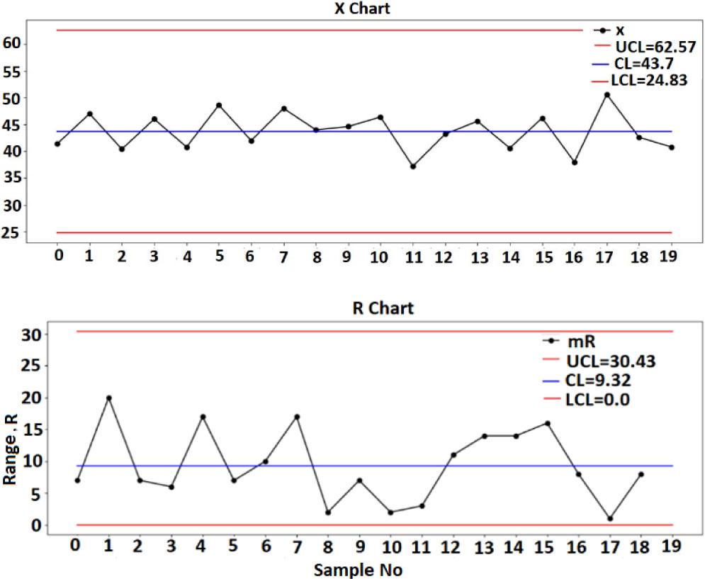
Example of X- and R-chart.
Table 2 presents the control chart constants (A2, A3, D3, D4, d2) used in constructing X̅- and R-charts. These constants are standard values published in SPC references.
Control chart constants (X̅- and R-charts).
| Sample size = m | A2 | A3 | d2 | D3 | D4 | B3 | B4 |
|---|---|---|---|---|---|---|---|
| 2 | 1.880 | 2.659 | 1.128 | 0 | 3.267 | 0 | 3.267 |
| 3 | 1.023 | 1.954 | 1.693 | 0 | 2.574 | 0 | 2.568 |
| 4 | 0.729 | 1.628 | 2.059 | 0 | 2.282 | 0 | 2.266 |
| 5 | 0.577 | 1.427 | 2.326 | 0 | 2.114 | 0 | 2.089 |
| 6 | 0.483 | 1.287 | 2.534 | 0 | 2.004 | 0.030 | 1.970 |
| 7 | 0.419 | 1.182 | 2.704 | 0.076 | 1.924 | 0.118 | 1.882 |
| 8 | 0.373 | 1.099 | 2.847 | 0.136 | 1.864 | 0.185 | 1.815 |
| 9 | 0.337 | 1.032 | 2.97 | 0.184 | 1.816 | 0.239 | 1.761 |
| 10 | 0.308 | 0.975 | 3.078 | 0.223 | 1.777 | 0.284 | 1.716 |
Note:
A2, A3 – factors for calculating control limits in X̅-chart;
D3, D4 – factors for calculating control limits in R-chart;
d2 – factor used to estimate standard deviation from range (σ ≈ R̅/d2);
B3, B4 – control chart constants used for constructing S-chart limits.
The X̅-chart is used to evaluate and control the accuracy of the measurement system, particularly in short-run applications, by analyzing subgroup mean values and assessing their closeness, consistency and statistical control.
Get N group of results (each group has n measurements).
Find the average values of each group from
(5) where n is the subgroup size (number of readings).\bar X = {{\sum {{X_i}} } \over n} = {{{x_1} + {x_2} + \cdots + {x_n}} \over n} Find the mid limit
{\bar {\bar {\bar X}}} (6) {\bar {\bar {\bar X}}} = {{\sum {{{\bar X}_i}} } \over N} = {{\overline {{x_1}} + \overline {{x_2}} + \cdots + \overline {{x_n}} } \over N} Find the UCL from
(7) {UCL}_x = \overline{\overline X} + {A_2}\bar R Find the LCL from
(8) where A2 is a control chart constant that depends on the subgroup size.{LCL}_x = \overline{\overline X} - {A_2}\bar R Plot the three limits, then add the values of X in-between the limits [5], [6].
The S-chart is employed to monitor process variability based on subgroup standard deviations. For each subgroup of n measurements, the standard deviation is calculated as:
The average subgroup standard deviation S̅ is then obtained across N subgroups:
Control limits for the S-chart are determined using constants B3 and B4, which depend on subgroup size:
UCL = B4 × S̅
CL = S̅
LCL = B3 × S̅
The S-chart provides a more reliable estimate of variability than the R-chart. In this study, the S-chart was used alongside the X̅- and R-charts to ensure comprehensive monitoring of both accuracy and precision during calibration.
This parameter provides an alternative estimate of process variability compared to the range-based method.
Having outlined the motivation and objectives of this study, the following section describes the experimental methodology applied at NIS.
The calibration of the platinum resistance thermometer (Pt-100) was performed at the NIS. The procedure involved the following steps:
A high-precision dry block furnace (Fluke model 9140, stability ±0.05 °C) was used to generate stable reference temperatures at 70 °C, 150 °C, and 200 °C.
A platinum resistance thermometer (Pt-100, four-wire configuration, IEC 60751 compliant) was used. This configuration eliminates the influence of lead wire resistance.
The platinum resistance thermometer (Pt-100) was connected to a precision resistance bridge (model CED7000) [7]. The bridge resistance readings were converted into temperature using the ITS-90 reference function for platinum resistance thermometers.
The platinum resistance thermometer (Pt-100) was positioned in the isothermal zone of the dry block furnace. At each set point (70 °C, 150 °C, 200 °C), the furnace was stabilized for at least 30 minutes before recording data.
At each point, 25 readings were collected (five groups of five repeated measurements). This design was chosen to provide a stronger statistical basis than the originally planned 20 readings, ensuring more reliable estimation of subgroup variability and enhancing the robustness of the control chart analysis. Reference data were compared with NIS traceable standards to validate measurement traceability.
The dry block furnace is specified with an accuracy of ±0.2 °C. However, at the 70 °C set point, deviations of up to 2.5 °C were observed. These deviations are attributed to:
Temperature gradients within the block, especially near the sensor insertion zone.
Sensor positioning: slight differences in immersion depth or contact can cause larger deviations at lower temperatures.
Calibration drift of the furnace's internal control sensor over time.
Environmental influences such as ambient fluctuations or heat losses.
To mitigate these effects, calibration results were always referenced to NIS traceable standards, and the observed deviations were incorporated into the uncertainty budget. While the furnace specification provides a nominal accuracy, the actual performance under laboratory conditions was treated as an additional source of uncertainty in the calibration process. Once the calibration procedure was established, the next step was to evaluate the associated measurement uncertainty and quality assurance aspects.
The overall calibration uncertainty of the Pt-100 resistance thermometer was evaluated in accordance with the Guide to the Expression of Uncertainty in Measurement (GUM). All relevant sources of uncertainty were identified, quantified, and combined to obtain the expanded uncertainty, as shown in Table 3. Each component was expressed as a standard uncertainty, then combined using the root-sum-of-squares method. The expanded uncertainty was calculated with a coverage factor k = 2, corresponding to a 95 % confidence level. The resulting calibration uncertainty is ±0.09 °C (k = 2), which ensures traceability and reliability of the calibration process [8],[9],[10],[11],[12].
The uncertainty budget of the platinum resistance thermometer (Pt-100) at 200 °C.
| Symbol | Source uncertainty | Value Xi ± (°C, Ω) | Divisor | Sensitivity coefficient | Uncertainty contribution | Method of estimation |
|---|---|---|---|---|---|---|
| Ust1 | Uncertainty of standard | 0.005 | 2 | 1 | 0.0025 | Calibration certificate |
| Ures | Resolution | 0.0001 | 3.46 | 1 | 2.88675E-05 | Digital indicator = 0.5 of resolution |
| Umul | Bridge | 0.0003 | 2 | 2.5 | 0.00037 | Calibration certificate |
| Udrf | Drift of bridge | 0 | 2 | 1 | 0 | Maximum difference between two successive calibrations of the standard |
| Ures uut | Resolution of UUT | 0.001 | 3.46 | 1 | 0.00028 | Digital indicator = 0.5 of resolution |
| Uaxi | Axial of dry block | 0.07 | 1.73 | 1 | 0.040 | Maximum difference between dry block holes for axial measurement |
| Urad | Radial of dry block | 0.04 | 1.73 | 1 | 0.023 | Maximum difference between dry block holes for radial measurement |
| Ustab | Stability of dry block | 0.05 | 3.46 | 1 | 0.0144 | Difference between maximum and minimum value of measurements |
| Uhyst | Hysteresis effects | 0.01 | 1.73 | 1 | 0.007 | Maximum difference between increase and decrease measurements |
| Urep | Repeatability (A) | 0.002 | 1 | 1 | 0.002 | Standard deviation of measurements |
| Combined uncertainty | 0.049 | |||||
| Expanded uncertainty | ± 0.09 oC |
Control charts (Shewhart X̅, R, and 3σ) were used to assess repeatability and reproducibility.
A Python-based automation algorithm was implemented to monitor live data, detect out-of-control points, and trigger alarms when deviations exceed permissible limits.
This methodology ensures traceability of measurements to national standards and provides statistical evidence of calibration reliability.
Provides continuous monitoring of calibration stability using control charts.
Detects systematic and random errors earlier than conventional calibration methods.
Enhances traceability by integrating SPC with national standards.
Reduces human error through automation and real-time alarms.
Improves confidence in calibration results by quantifying repeatability and reproducibility.
Requires larger datasets (multiple subgroups) compared to conventional single-point calibration.
Assumes stable environmental conditions; sensitive to external disturbances.
Implementation of SPC and automation requires specialized software and statistical expertise.
The method is best suited for routine calibration laboratories; it may not be practical for quick field calibrations.
To assess the statistical behavior of the Pt-100 calibration data, a subgroup analysis was first performed. For each calibration setting, multiple subgroups of repeated readings were collected, and their means (X̅), ranges (R), and standard deviations (S) were calculated. These subgroup statistics were then used to estimate the overall process parameters and to establish the corresponding control chart limits.
To evaluate the stability and consistency of the Pt-100 calibration process, statistical control charts were constructed based on subgroup data. The analysis included the X̅-chart for monitoring subgroup means, the R-chart for subgroup ranges, and the S-chart for subgroup standard deviations. These charts provide a comprehensive assessment of both the process average and inherent variability, enabling detection of out-of-control conditions or unusual trends over time. By integrating the subgroup data with the calculated control limits, both the tables and the control charts provide a clear picture of the process stability and variability over time.
Table 4 presents the raw calibration readings of the Pt-100 thermometer at three reference temperatures (200 °C, 150 °C, and 70 °C). For each setting, five subgroups were recorded, with five repeated measurements per subgroup.
The raw calibration readings of Pt-100 thermometer at (200 °C, 150 °C, and 70 °C).
| Setting | Groups | Reading [°C] | ||||
| 1 | 2 | 3 | 4 | 5 | ||
| 200 °C | 1 | 200.4 | 200.5 | 200.5 | 200.4 | 200.5 |
| 2 | 200.6 | 200.6 | 200.5 | 200.5 | 200.6 | |
| 3 | 200.3 | 200.5 | 200.4 | 200.6 | 200.7 | |
| 4 | 200.6 | 200.5 | 200.5 | 200.4 | 200.6 | |
| 5 | 200.3 | 200.4 | 200.6 | 200.5 | 200.5 | |
| Setting | Groups | Reading [°C] | ||||
| 1 | 2 | 3 | 4 | 5 | ||
| 150 °C | 1 | 148.8 | 148.6 | 148.7 | 148.8 | 148.5 |
| 2 | 148.7 | 148.6 | 148.5 | 148.7 | 148.6 | |
| 3 | 148.7 | 148.6 | 148.8 | 148.7 | 148.7 | |
| 4 | 148.9 | 148.7 | 148.8 | 148.7 | 148.6 | |
| 5 | 148.7 | 148.8 | 148.7 | 148.6 | 148.7 | |
| Setting | Groups | Reading [°C] | ||||
| 1 | 2 | 3 | 4 | 5 | ||
| 70 °C | 1 | 67.5 | 67.6 | 67.5 | 67.3 | 67.5 |
| 2 | 67.7 | 67.6 | 67.5 | 67.4 | 67.6 | |
| 3 | 67.3 | 67.5 | 67.4 | 67.6 | 67.7 | |
| 4 | 67.6 | 67.7 | 67.5 | 67.4 | 67.6 | |
| 5 | 67.2 | 67.4 | 67.6 | 67.6 | 67.5 | |
This structure of data collection allows both the estimation of the subgroup mean (X̅), range (R), and standard deviation (S), and the subsequent construction of control charts (X̅, R, and S). The repeated measurements at each setting reduce random error, while the use of multiple subgroups provides a reliable basis for estimating process variability and stability.
The results demonstrate that the readings are closely clustered around their nominal values, with only minor fluctuations, indicating high repeatability of the calibration process.
Table 5 combines both the subgroup statistics and the calculated control chart limits for the Pt-100 calibration. For each subgroup, the mean (X̅), range (R), and standard deviation (S) were determined, allowing the estimation of process variability. The overall averages (X̿, R̅, S̅) were then used, together with the standard SPC constants (A2, D3, D4, B3, B4), to calculate the control limits of the X̅, R, and S-charts.
Control charts, constants, and calculated limits for Pt-100 calibration subgroup statistics.
| X̅ | R | S | σ | X̿ | R̅ | S̅ |
|---|---|---|---|---|---|---|
| 67.48 | 0.3 | 0.109544512 | 0.130128142 | 67.512 | 0.34 | 0.126802209 |
| 67.56 | 0.3 | 0.114017543 | ||||
| 67.50 | 0.4 | 0.129099445 | ||||
| 67.56 | 0.3 | 0.114017543 | ||||
| 67.46 | 0.4 | 0.167332005 |
| A2 | B3 | B4 | D3 | D4 | X̅UCL | X̅LCL | RUCL | RLCL | SUCL | SLCL |
|---|---|---|---|---|---|---|---|---|---|---|
| 0.577 | 0 | 2.089 | 0 | 2.114 | 67.69664 | 67.32736 | 0.718 | 0 | 0.2681 | 0 |
This integrated presentation presents both observed subgroup variation and statistical control limits in a single table, simplifying interpretation and clearly demonstrating that all subgroup means remain within the calculated control boundaries, confirming the statistical stability of the calibration process.
Table 6 indicates calibration readings of the Pt-100 thermometer with calculated mean, warning limits UWL/LWL = ±2σ, and control limits UCL/LCL = ±3σ. The data presented in Table 6 show that all calibration readings of the Pt-100 thermometer over the period 2021–2024 remain within the statistical control limits (UCL = 67.902 °C, LCL = 67.122 °C).
The calculated control limits for the platinum resistance thermometer (Pt-100) calibration process over multiple years.
| Date | Reading [°C] | X̿ [°C] | 1σ | 2σ | 3σ | 1σ | 2σ | 3σ |
|---|---|---|---|---|---|---|---|---|
| UWL [°C] | LWL [°C] | |||||||
| 20 March 2021 | 67.48 | 67.512 | 67.64212814 | 67.77225628 | 67.90238443 | 67.38187186 | 67.25174372 | 67.12161557 |
| 20 June 2021 | 67.60 | 67.512 | 67.64212814 | 67.77225628 | 67.90238443 | 67.38187186 | 67.25174372 | 67.12161557 |
| 12 September 2021 | 67.42 | 67.512 | 67.64212814 | 67.77225628 | 67.90238443 | 67.38187186 | 67.25174372 | 67.12161557 |
| 22 December 2021 | 67.56 | 67.512 | 67.64212814 | 67.77225628 | 67.90238443 | 67.38187186 | 67.25174372 | 67.12161557 |
| 22 March 2022 | 67.54 | 67.512 | 67.64212814 | 67.77225628 | 67.90238443 | 67.38187186 | 67.25174372 | 67.12161557 |
| 22 June 2022 | 67.50 | 67.512 | 67.64212814 | 67.77225628 | 67.90238443 | 67.38187186 | 67.25174372 | 67.12161557 |
| 22 September 2022 | 67.60 | 67.512 | 67.64212814 | 67.77225628 | 67.90238443 | 67.38187186 | 67.25174372 | 67.12161557 |
| 22 December 2022 | 67.50 | 67.512 | 67.64212814 | 67.77225628 | 67.90238443 | 67.38187186 | 67.25174372 | 67.12161557 |
| 19 March 2023 | 67.56 | 67.512 | 67.64212814 | 67.77225628 | 67.90238443 | 67.38187186 | 67.25174372 | 67.12161557 |
| 19 June 2023 | 67.48 | 67.512 | 67.64212814 | 67.77225628 | 67.90238443 | 67.38187186 | 67.25174372 | 67.12161557 |
| 19 September 2023 | 67.42 | 67.512 | 67.64212814 | 67.77225628 | 67.90238443 | 67.38187186 | 67.25174372 | 67.12161557 |
| 22 December 2023 | 67.60 | 67.512 | 67.64212814 | 67.77225628 | 67.90238443 | 67.38187186 | 67.25174372 | 67.12161557 |
| 19 March 2024 | 67.46 | 67.512 | 67.64212814 | 67.77225628 | 67.90238443 | 67.38187186 | 67.25174372 | 67.12161557 |
| 25 June 2024 | 67.54 | 67.512 | 67.64212814 | 67.77225628 | 67.90238443 | 67.38187186 | 67.25174372 | 67.12161557 |
| 25 September 2024 | 67.60 | 67.512 | 67.64212814 | 67.77225628 | 67.90238443 | 67.38187186 | 67.25174372 | 67.12161557 |
| 19 December 2024 | 67.50 | 67.512 | 67.64212814 | 67.77225628 | 67.90238443 | 67.38187186 | 67.25174372 | 67.12161557 |
The process mean was calculated as 67.512 °C, with warning limits at ±2σ (UWL = 67.772 °C, LWL = 67.252 °C). Since all points lie inside the ±3σ boundaries, the process is statistically stable and no out-of-control condition is observed. Furthermore, all readings fall within the ±2σ warning limits, indicating a high level of process consistency and calibration reliability over time.
To clarify their practical use during calibration, the X̅- and R-charts are constructed from a set of preliminary calibration measurements (baseline data). These initial measurements establish the process mean and the control limits for both charts. During subsequent calibration cycles, each new series of repeated measurements is plotted on the established X̅- and R-charts. The new subgroup mean is evaluated against the X̅-chart limits, while the within-subgroup variation is assessed using the R-chart.
If any new point violates the Shewhart or Westgard rules, such as a mean falling outside the limits, an abnormal increase in range, or the appearance of non-random patterns, the calibration run is flagged for investigation. This may require repeating the measurements, checking sensor stability, or evaluating environmental or procedural factors.
Thus, these charts serve as real-time decision tools during calibration: preliminary data are used to set the limits, and all later calibration series are assessed against them to ensure the measurement system remains statistically stable.
The calculated subgroup statistics and control limits presented in the tables served as the basis for constructing the X̅, R, and S control charts, which provide a graphical representation of process stability and variability.
Fig. 2, Fig. 3, and Fig. 4 present the control charts used to evaluate the stability of the Pt-100 calibration process.
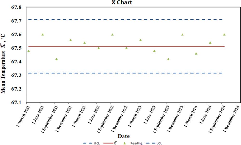
X̅ control chart for Pt-100 calibration readings.
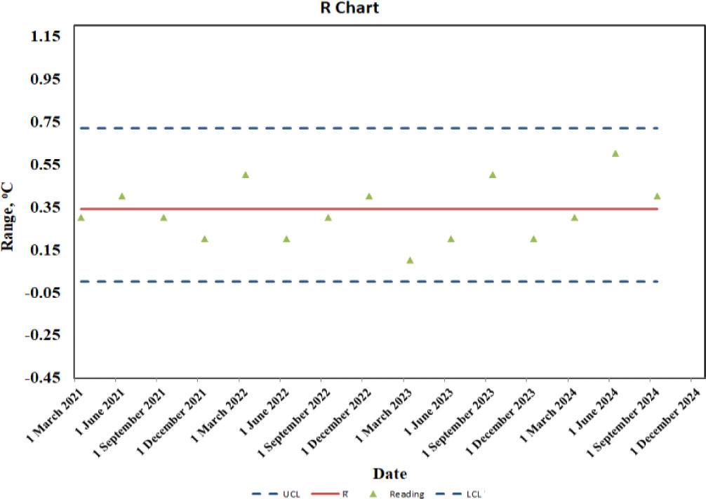
R control chart for Pt-100 calibration readings.
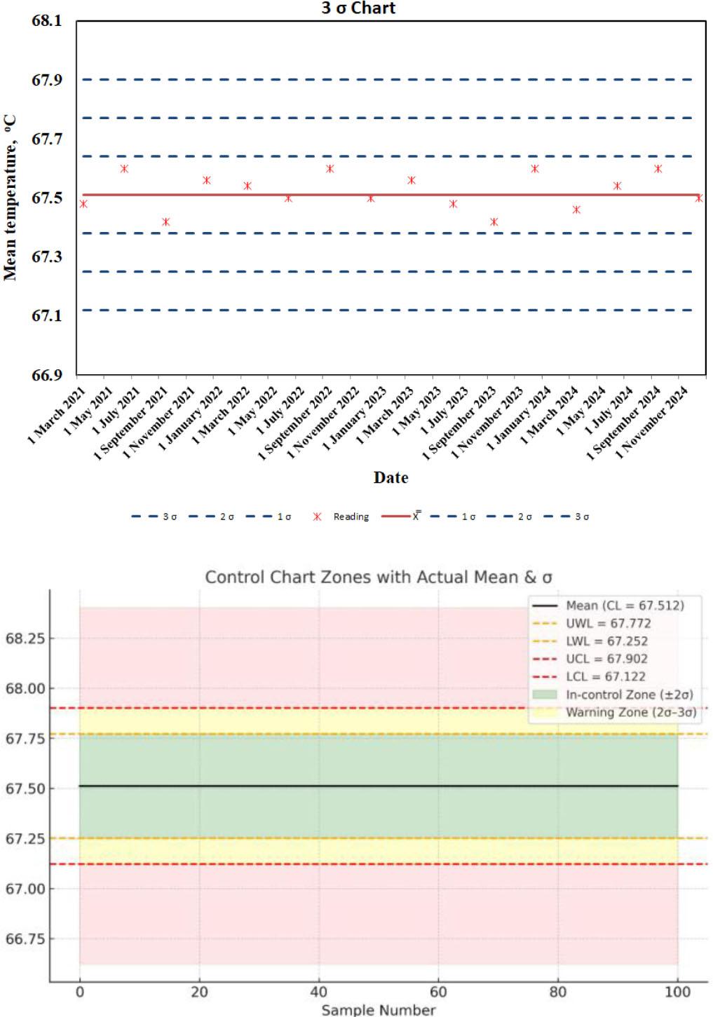
3σ̂ (estimated from sample data) chart for Pt-100 calibration readings.
Each figure corresponds to a specific chart type and is explained below. These charts are not only descriptive but also serve as decision tools during calibration.
Fig. 2 – X̅-chart: This chart monitors subgroup means. In this study, all subgroup means remained within the calculated control limits (UCL = 67.7 °C, LCL = 67.3 °C) and centered around the process mean of 67.5 °C. This confirms that the overall calibration process average is statistically stable.
Fig. 3 – R-chart shows the subgroup ranges, which fall consistently within their control limits. The observed ranges (≈0.0–0.67 °C) confirm minimal short-term variation between repeated readings, indicating good measurement precision.
Fig. 4 represents the 3-sigma Shewhart chart constructed from the individual calibration readings. The subgroup standard deviations are ≈0.0–0.26 °C. All points lie within the ±3σ control limits with no trends or rule violations, confirming that the overall process variability is low and that the calibration system remained in statistical control throughout the study period.
Together, these charts provide a comprehensive monitoring framework:
- ▪
Preliminary calibration data are used to construct the charts and establish control limits.
- ▪
Subsequent calibration series are then compared against these limits.
- ▪
If any point violates the Shewhart or Westgard rules, the calibration run is flagged as potentially invalid, prompting either repetition of measurements or investigation of the instrument under test.
- ▪
The absence of out-of-control points in all three charts verifies that the calibration process remained statistically in control and highly reliable over the monitoring period.
The three charts show that both the mean and the variability remained stable, with no Shewhart or Westgard rule violations observed.
Building on the results obtained, the following section introduces the Python-based algorithm developed to automate statistical analysis and real-time monitoring.
References [13],[14],[15],[16] provide supporting background on statistical methods, uncertainty propagation, and control applications in similar measurement and calibration systems.
To ensure the continuity of quality measurements, we developed a Pythonic script, an open-source code used in the Python and Jupyter notebook environments. The code is free for all readers to use as follows.
This software is capable to:
Automatically acquire, handle, and store the collected data from live measurements.
Visualize the data density, and extract and compare the median, mode, and mean.
Estimate the variance and standard deviation
Calculate the UWL, UWL = μ + 2σ
Calculate the LWL, LWL = μ − 2σ
Calculate the UCL, UCL = μ + 3σ
Calculate the LCL, LCL = μ − 3σ
These limits are calculated using the process mean μ ± kσ, where k is a factor typically equal to 2. They provide early warning signals before the control limits are reached. Points falling between the warning limits and the control limits may indicate a potential shift in the process and should be monitored carefully. These are warning or alert limits and not official specification limits.
These are the main statistical limits on a control chart. They are typically calculated at ±3 standard deviations (σ) from the process mean. Any point beyond these limits signals that the process is out of statistical control and usually indicates the presence of a special-cause variation that must be investigated. They are usually set at ±2 standard deviations (σ) from the mean: If a point falls between 2σ and 3σ (i.e., between UWL and UCL or between LWL and LCL), the process is still considered in control, but this is a warning zone. Repeated points in this zone suggest the process may be drifting toward instability. It helps detect issues earlier, before they trigger a full out-of-control condition.
UCL/LCL (±3σ): Out-of-control detection;
UWL/LWL (±2σ): An early warning system alerts to potential problems before the process goes out of control.
The benefit of the Python-based algorithm shown in Appendix lies in automating the entire process, from data acquisition to three possible outputs: stop, alarm, or continue. This enables us to control the measurement fully and continually monitor the process. The simplicity and, at the same time, strong Pythonic algorithm facilitate the measurements and allow immediate judgement during live measurements, without long calculations each time. The Python script also includes a plotting module that automatically generates control charts, enabling real-time monitoring and detection of any out-of-control conditions. This automation ensures accuracy, saves analysis time, and minimizes the possibility of human error in manual calculations.
This study demonstrated the application of SPC methods in the calibration of a platinum resistance thermometer (Pt-100). By analyzing calibration data using subgroup statistics and constructing the X̅, R, and S control charts, the stability and repeatability of the calibration process were verified. All subgroup means and variability measures were found to lie within the calculated control limits, indicating that the process remained statistically in control throughout the monitoring period and confirmed that the calibration results consistently met the required specification limits, with minimal variation. The integration of the Python code to automate the statistical analysis and chart generation improved the reliability and reproducibility of the results. Overall, the findings confirm that the calibration process of the platinum resistance thermometer (Pt-100) is both accurate and stable, and the adopted methodology can serve as a framework for improving calibration quality assurance in similar measurement systems.
The inclusion of a Python-based monitoring program enables real-time detection of deviations, saving time and improving accuracy. This approach can be used as a model for other calibration laboratories seeking to strengthen their quality assurance systems. Python code will trigger an alarm to indicate an issue and stop the measurement process. This methodology can be adopted by other calibration laboratories to improve quality assurance and minimize human errors. Future work will extend this methodology to other types of thermometers and measurement systems to generalize its applicability.