
With an aging population, more people suffer from damaged hip joints caused by diseases and physical activities, making total hip arthroplasty (THA) — also known as total hip replacement (THR) — the most reliable resort to regain full mobility and alleviate the pain [1]. According to the 2023 Annual Report from the American Joint Replacement Registry (AJRR), approximately 544000 hip replacements are performed in the US annually, with projections soaring to 850000 by 2030 and 1429000 by 2040 [2], [3].
The THA procedure can be briefly summarized into three steps as shown in Fig. 1:
first, resect the diseased femoral head and debride the acetabulum;
second, implant the acetabular cup and femoral head prosthesis; and
finally, verify the joint mobility and stability prior to incision closure.
Among these steps, the precise placement of the acetabular cup within the “safe zone” — defined as an inclination angle of 40°±10° and an anteversion angle of 15°±10° [4] — is paramount to surgical success [5], [6]. Deviations from the “safe zone” can lead to serious complications, including dislocation, prosthetic impingement, accelerated wear, leg length discrepancy, and bearing-related noise [7].
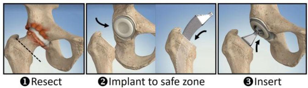
Overview of the three steps in the THA procedure.
Given the clinical significance of cup orientation, numerous technologies have been developed to guide intraoperative cup placement. Traditional tools such as mechanical alignment guides (MAGs) and protractors are common and cost-effective but highly dependent on surgeons' clinical experience, as they provide only passive visual references for surgeons without offering objective feedback [8]–[10]. Computer and robotic navigation systems are currently the most precise methods with a displacement error within 1 mm and an angular error within 1°, but suffer from high complexity, elevated costs, preoperative radiation expo-sure, and invasive bony marker insertion that increases bone damage and pin tract-related complication risks [11], [12]. These two types of technologies are currently the most widely adopted.
With the recent advancements in inertial measurement units (IMUs), IMU-based technologies have emerged as a key research trend. The IMU-based inclinometers can provide real-time, accurate, radiation-free intraoperative navigation with simplicity and portability, but most still require bony pin fixation and lack detailed descriptions of their measurement mechanisms [13], [14]. Gu et al. proposed a portable inertial navigation system for THA, achieving a root mean square error (RMSE) of 1.24° for radiographic anteversion and 1.89° for radiographic inclination, but only targeting the direct anterior approach [15]. Chen et al. proposed an IMU-based real-time measuring system for acetabular prosthesis implant angles, but it has low measurement accuracy (RMSE of inclination: 3.26°; anteversion: 3.05°) and poor clinical adaptability [16]. Tang et al. developed an IMU-based smart hip trial system and verified its performance via in vitro sawbone tests, yet it requires sensor integration into prostheses and has limited prosthesis adaptability [17].
To address the limitations of the current technologies, this paper proposes an intraoperative IMU-based method for measuring acetabular cup inclination and anteversion in THA, with the core objective of guiding precise cup placement within the safe zone. The method integrates an IMU-based pose estimation device, a non-invasive registration strategy, and a robust two-phase workflow (registration and measurement). Unlike traditional IMU-based approaches, the proposed method is a non-invasive, radiation-free, low-cost, and portable solution that is independent of bony anatomical landmarks and IMU mounting poses.
Real-time measurement of acetabular cup inclination and anteversion is key to ensuring its positioning within the safe zone. There are several different definitions of the inclination and anteversion angles, including operative, radiographic, and anatomical definitions [18]. In this paper, the operative inclination θi and anteversion θa are the selected definitions, which are illustrated in Fig. 2(a).
To mathematically describe the inclination and anteversion of the acetabular cup, a human body coordinate system (abbreviated as {B}) is first established. The system {B} is built using the coronal, sagittal, and horizontal planes of the human body, with its positive x-axis defined as the direction orthogonal to the sagittal plane and pointing to the body’s right, the positive y-axis as the direction orthogonal to the coronal plane and pointing forward, and the positive z-axis as the vertical upward direction along the spinal axis, as shown in Fig. 2(b).
Then the cup axis (normal vector of the cup) in {B} is used to represent the orientation of the acetabular cup, as shown by the red line in Fig. 2(b). Assume that n is a vector along the cup axis, whose orientation is actually determined by the inclination and anteversion. Its coordinates can be expressed as in (1),
As the inclination θi and anteversion θa are angles defined on the coronal and horizontal planes, respectively, the vector n is finally projected onto the coronal and horizontal planes to find the equivalent angles for θi and θa. The projection results are shown by the blue and brown lines in Fig. 2(b), and can be expressed as (2).
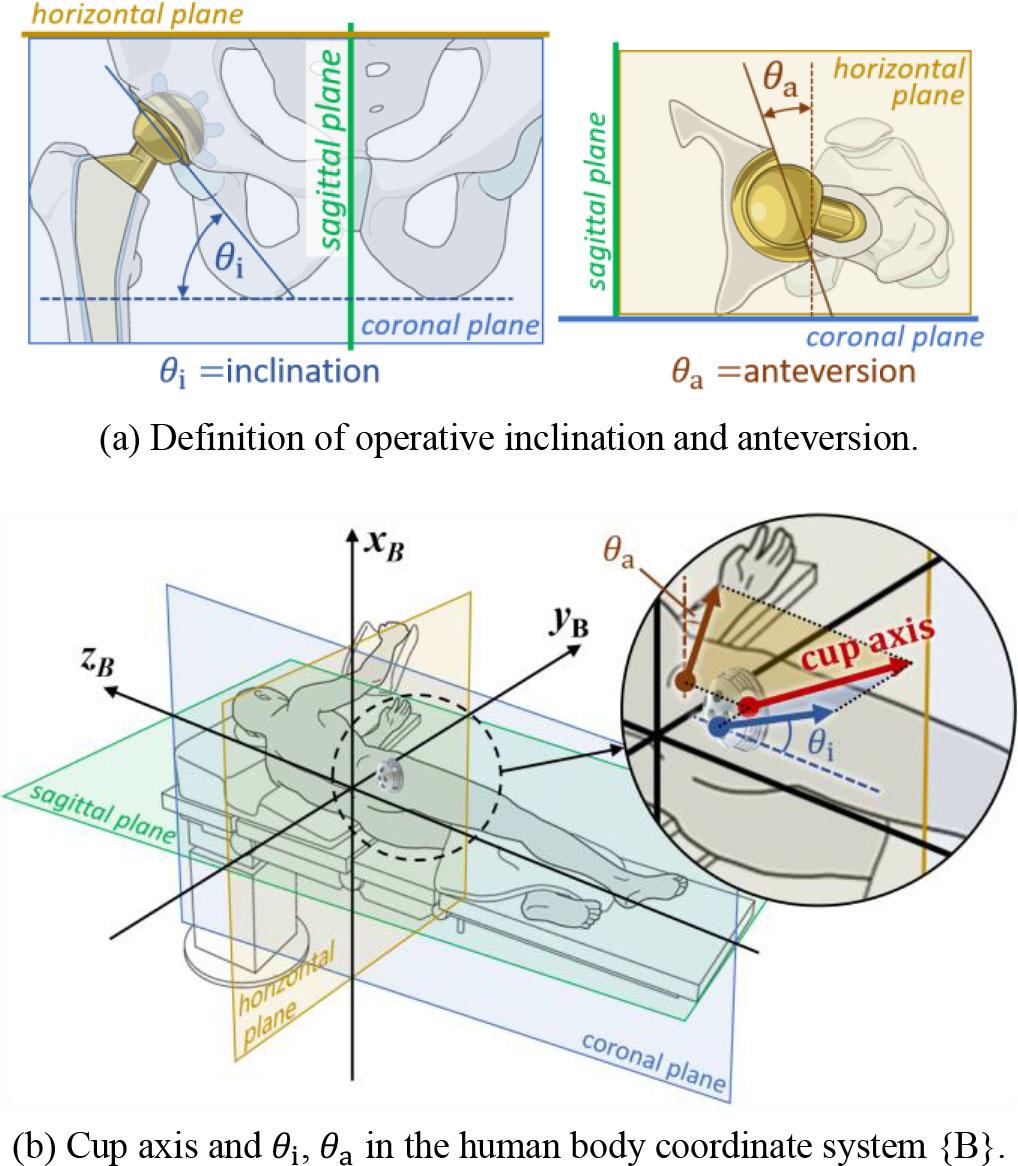
Definitions of operative inclination θi, anteversion θa, and human body coordinate system {B}, and the illustration of cup axis and equivalent angles for θi and θa in system {B}.
According to geometric relationships, the inclination θi equals the angle between the projection
Now the problem of measuring θi and θa has been transformed into the acquisition of the coordinates of vector n in {B}. To achieve this, the world system {W} and the IMU sensor system {I} are defined as shown in Fig. 3. The East-North-Up (ENU) system is used as the definition of {W}, while a body-fixed coordinate system is used as {I}. The definitions of {W}, {I}, and {B} are summarized in Table 1.
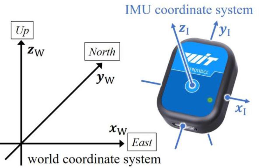
Definitions of the IMU coordinate system {I} and the world coordinate system {W}.
Definitions of the three coordinate systems: world system{W}, IMU system {I}, and body system {B}.
| Name & notation | Definition |
|---|---|
| World | xW: pointing east |
| system | yW: pointing north |
| {W} | zW: pointing up, orthogonal to the local Earth surface |
| IMU | xI: pointing right (viewing from front-facing direction) |
| system | yI: pointing up (viewing from front-facing direction) |
| {I} | zI: pointing forward (front-facing direction) |
| Body | xB: pointing to the body’s right |
| system | yB: pointing forward |
| {B} | zB: pointing up along the spinal axis |
The orientation of a rigid body in a 3D reference coordinate system can be described by the relative orientation between its own coordinate system and the reference coordinate system. Several mathematical tools exist for this purpose [19], including rotation matrices, Euler angles, quaternions, etc. These tools can be transformed into each other. In this paper, a combined approach using rotation matrices and Euler angles is applied to describe the relative orientation of coordinate systems, which is intuitive and easy to understand.
The rotation matrix is a fundamental tool for describing the rotation of a rigid body. Rotation about a single axis of the coordinate system is called elementary rotation, and any rotation can be decomposed into a combination of elementary rotations about three axes [20]. The elementary rotation by angle α about the x-axis is represented by a rotation matrix Rx(α) as shown in (4).
Similarly, rotation by angle β about the y-axis and rotation by angle γ about the z-axis are the other two elementary rotations and can also be represented by Ry(β) and Rz(γ) as shown in (5) and (6), respectively.
There are two different ways to define the composition of multiple elementary rotations, namely extrinsic rotations and intrinsic rotations [21]. Extrinsic rotations refer to rotations that are applied to a space-fixed coordinate system. When composing extrinsic rotations, the order of rotations is crucial. For example, applying extrinsic rotations in the order of (R0,R1,⋯,Rn) results in a net rotation Re as shown in (7).
In contrast, intrinsic rotations involve applying each rotation about the axes of the current coordinate system (also known as a body-fixed coordinate system), which is dynamically updated after each rotation. When combining multiple intrinsic-type elementary rotations into a net rotation, the order of matrix multiplication is the opposite of that for extrinsic rotations. For example, the net rotation Ri from a series of intrinsic rotations in the order of (R0,R1,⋯,Rn) can be expressed as (8), where the matrix multiplication order follows the sequence of rotations.
In 1776, Leonhard Euler proposed Euler angles, which describe the relative orientation of coordinate systems by decomposing the rotational transformation into elementary rotations about three axes [22]. In this paper, the Euler angles, known as Tait-Bryan angles, are used, which were proposed by Peter Guthrie Tait and George H. Bryan in the 19th century. These Euler angles, denoted as (α,β,γ), decompose the rotation of a rigid body into three sequential elementary rotations, as shown in (9),
Based on this equation, the inverse transformation from rotation matrices to Euler angles (solution for β in the range (−π/2,π/2)) can also be derived, as shown in (10),
In addition to describing rotational movement, a rotation matrix also represents the coordinate transformation relationship before and after rotation. In the IMU-based solution, Euler angles are the output of the IMU sensor and are converted to the rotation matrix, denoted as
In the previous problem definition, the measurement of cup orientation has been transformed into the acquisition of the coordinates of the unit vector n along the cup axis in {B}. However, since an IMU can only measure orientation with respect to {W}, acquiring the cup’s orientation requires two steps: registration and measurement. The goal of registration is to establish the transformation relationship between systems {B} and {W}, while the measurement is to first obtain the coordinates nW in {W}, then convert them into nB in {B}, and finally calculate the cup inclination and anteversion using (3).
Assuming the patient and the operating table remain relatively immobile throughout the surgery, the orientation of the operating table can be used to represent the patient's body orientation. For ease of discussion, take the left lateral decubitus position shown in Fig. 2(b) as an example. Since the operating table is horizontally placed, the xB-axis is considered parallel to the zW-axis, meaning that:
Thus, the transformation relationship between {B} and {W} can be determined if the orientation of the yB-axis or the zB-axis is acquired. During registration, an IMU is used to measure the coordinates of the unit vector eBz in {W} along the zB-axis, which is parallel to the long axis of the operating table. The IMU is mounted on the operating table in any orientation, and the operating table is rotated about its long axis by a small angle (about 10°). By recording the Euler angles from IMU before and after rotation, the axis of this rotation — i.e., the zB-axis — can be obtained. Suppose (α1,β1,γ1) and (α2,β2,γ2) are the Euler angles from the IMU before and after rotation, respectively; the relative rotational transformation can be derived from (9) and (12) as shown in (14).
Convert the rotational matrix
At this point, the orientations of the xB-axis and the zB-axis are both obtained, so the coordinates of the unit vector along the yB-axis in {W} are derived from (13) and (17), as shown in (18).
According to the definition of the rotation matrix, the transformation matrix
With the transformation relationship
During this phase, an IMU is mounted on the acetabular cup axis with a specific orientation to measure the cup's inclination and anteversion. Mount the IMU on the acetabular cup impactor such that the x-o-y plane of the IMU coordinate system {I} is perpendicular to the acetabular cup axis. In this case, the axis of the acetabular cup can be represented by the z-axis of {I}. Let n denote the axial vector along the cup axis as shown in (1), so n = eIz, and its coordinates in {I} are as shown in (20).
During the THA procedure, the IMU mounted on the cup axis can measure and output the Euler angles (αc,βc,γc), so the real-time orientation of {I} relative to {W}, denoted as
Since the transformation matrix of {B} relative to {W} has been established during the registration phase, as given by (19), combining it with (22) yields the coordinates of n in {B}, as shown in (23).
The coordinates nB = (nxB,nyB,nzB)T of the vector n in {B} have been obtained at this point. As previously analyzed in (2) and (3) in the problem definition section, the inclination θi and anteversion θa of the acetabular cup can finally be computed using (3), and the measurement phase is finished.
To validate the effectiveness of the method, a 3-axis tilt table is used, as shown in Fig. 4. This precision instrument consists of three layers: the bottom two are formed by two orthogonally stacked single-axis tilt tables, and the third layer is a circular turntable that can rotate 360° about its vertical axis. Each layer is equipped with a main scale and a vernier sub-scale to improve angular reading accuracy, achieving a resolution of 0.1°. A threaded rod with an acetabular cup attached at one end is vertically screwed into the center of the circular turntable to simulate the cup axis during surgery. The parameters of the experimental equipment are as follows:
Tilt table:
rotation range (x/y-axis: ±40°, z-axis: 360°);
resolution (0.1°);
repeat positioning accuracy (±0.05°);
load capacity (5 kg).
IMU:
sensor model (MPU9250);
sampling rate (200 Hz);
accelerometer accuracy (±0.01 g);
gyroscope accuracy (±0.005°/s).
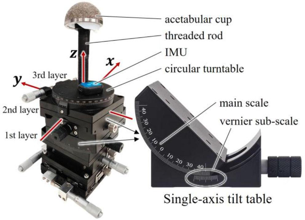
The full view image of the 3-axis tilt table used in experiments (left) and the close-up image of the single-axis tilt table (right), which is the constituent unit of the bottom two layers. The threaded rod simulates the axis of the acetabular cup.
This instrument can simulate both extrinsic rotation and intrinsic rotation in three dimensions. According to the three-layer stacked structure shown in Fig. 4, the following interactions exist among the three rotational axes:
Rotation about the z-axis does not affect the y-axis or x-axis;
Rotation about the y-axis causes the z-axis to change accordingly;
Rotation about the x-axis causes both the z-axis and y-axis to change accordingly.
As a result, when using this instrument, rotating in the z-y-x axis order corresponds to extrinsic rotation, while rotating in the x-y-z order corresponds to intrinsic rotation. The experiments conducted with this instrument are as follows.
This experiment aimed to test the fundamental functionality of the IMU used in this paper, i.e., its performance in estimating its own rotational angles. The IMU was mounted on the 3-axis tilt table at an arbitrary initial orientation. The tilt table was then directed to perform a series of rotations: it was first rotated about the z-axis from 0° to 20° and then in the reverse direction to −20°, with the measured values (true values) from the tilt table and the estimated values from the IMU recorded at every 5° intervals; subsequently, the identical rotation procedure and data recording were conducted for the y-axis and x-axis, respectively. The results and the errors are shown in Fig. 5.
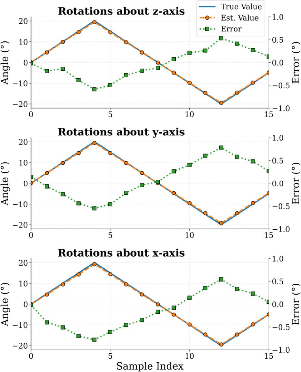
Angle estimation accuracy of the IMU for single-axis rotation. The true values (blue line) and estimated values (orange line) are referenced to the left vertical axis, while their absolute errors (green line) are referenced to the right vertical axis.
The results demonstrated that, irrespective of the rotation axis, the estimated angles were in good agreement with the true ones, and the absolute errors stayed within ±1°. Importantly, the magnitude of error showed a clear trend of increasing with the rotation angle. The error is attributed to three primary factors: IMU sensor intrinsic noise, the data fusion latency, and mechanical jitter during rotation. RMSE and mean absolute percentage error (MAPE) were acquired as shown in (24) and (25), and were listed in Table 2 to evaluate the angle estimation accuracy.
Angle estimation accuracy (using RMSE and MAPE) of rotations in the three axes.
| Rotation axis | RMSE | MAPE |
|---|---|---|
| z-axis | 0.315° | 2.5 % |
| y-axis | 0.409° | 3.3 % |
| x-axis | 0.423° | 3.6 % |
In the registration phase, establishing the transformation between coordinate systems {B} and {W} depends on accurately acquiring the orientation of the z-axis of {B} by rotating the operating table. Therefore, the goal of this experiment was to test how well the rotation axis coordinates can be acquired. In the experiment, the IMU was attached to the turntable of the 3-axis tilt table. The tilt table was then rotated about its y-axis to simulate the operating table’s rotation about its long axis during the registration phase, and our method estimated the coordinates of the unit vector along this rotation axis. An algorithm computed and recorded the rotation axis vector coordinates for this movement after the IMU sent the Euler angle data (before and after rotation) to the PC via Bluetooth.
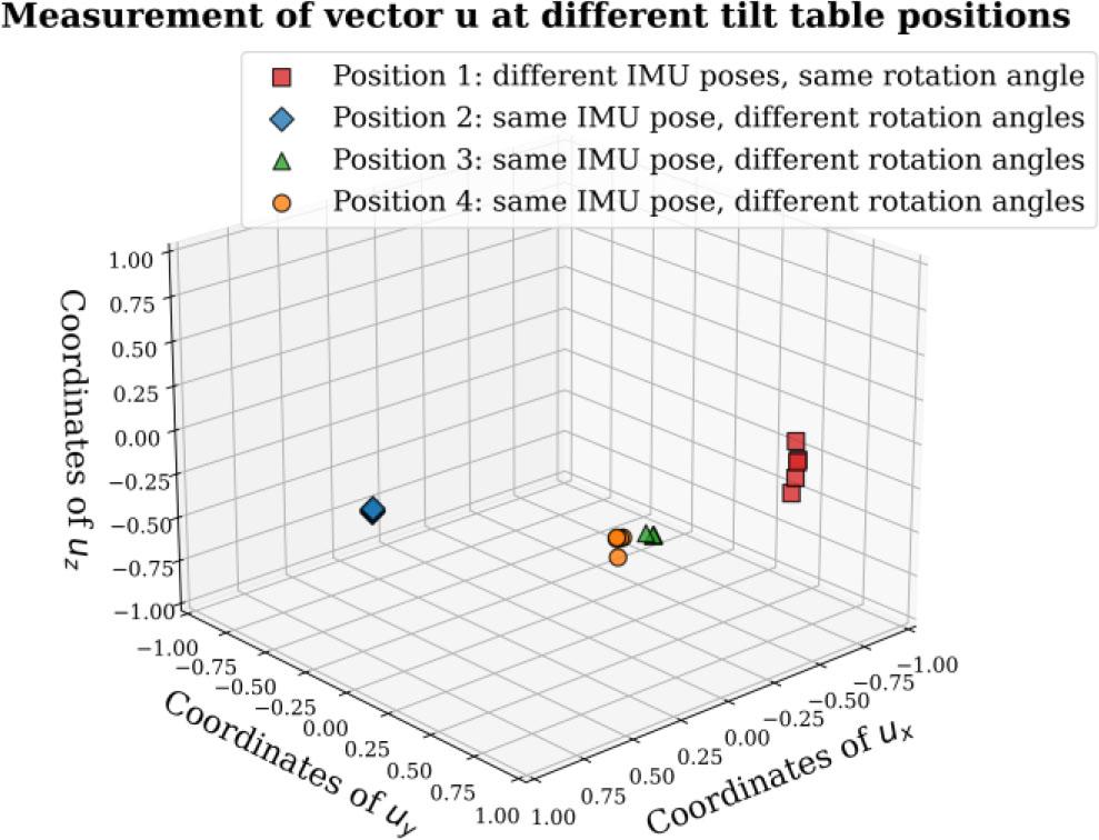
Coordinates of rotation axis unit vector uW in {W} acquired during the registration phase using (17), recorded at four positions.
The tilt table was positioned at four different locations on the test tabletop for the experiment. In multiple measurements at Position 1, the tilt table rotated by a fixed 10° about its y-axis, but the IMU was secured to the tilt table in varying poses each time to test whether the IMU pose affects the rotation axis vector acquisition. For Positions 2–4, the IMU remained in a consistent pose, while the tilt table’s rotation angles about the y-axis varied from 3° to 15°, aiming to investigate the effect of rotation angle. The rotation axis vector coordinates obtained at different tilt table positions, IMU orientations, and rotation angles are plotted in a scatter plot (Fig. 6).
Since the tilt table sits on the test table, its y-axis remains almost horizontal. For the estimated rotation axis vector coordinates
Part of the data (estimated coordinates of rotation axis vector at Position 1 & 2) and the corresponding test conditions (IMU pose & rotation angle).
| Tilt table position | IMU pose | Rotation angle | Estimated axis vector
|
|---|---|---|---|
| Position 1 | Pose A | 10° | (−0.586, 0.810, −0.024) |
| Pose B | (−0.565, 0.819, 0.103) | ||
| Pose C | (−0.579, 0.808, −0.111) | ||
| Pose D | (−0.601, 0.799, −0.022) | ||
| Pose E | (−0.553, 0.812, −0.186) | ||
| Position 2 | Pose A | 3° | ( 0.993, 0.119, 0.020) |
| 6° | ( 0.993, 0.120, 0.006) | ||
| 9° | ( 0.993, 0.119, 0.006) | ||
| 12° | ( 0.993, 0.117, −0.004) | ||
| 15° | ( 0.994, 0.114, 0.007) |
To verify the accuracy of our method, the 3-axis tilt table was used to simulate the human body coordinate system, while the threaded rod screwed into the center served as the acetabular cup axis, representing the implantation angle of the cup. Through geometric derivation, the cup's θi and θa were converted into the tilt table’s rotation angles about its x-axis and y-axis, respectively.
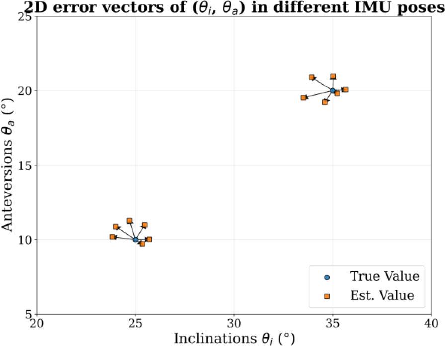
The experiment began after the registration was done. The IMU was fixed on the top circular turntable, facing up to ensure its zI-axis was parallel to the cup axis. Then the tilt table was rotated about its x-axis and y-axis to move the cup axis to a series of preset orientations (changing from (25°, 5°) to (40°, 20°) at 5° intervals). Meanwhile, the PC received real-time Euler angle data from the IMU and immediately estimated the current θi and θa. The experimental results were saved as 2D vectors (θi,θa) and plotted on a 2D coordinate graph, as shown in Fig. 7.
Comparison of estimated (θi,θa) values vs. true values. A larger magnitude of the error vector indicates greater error.
The measurement accuracy was evaluated by the RMSE of both angles and the magnitude of the error vector, i.e.,
Results of θi and θa measurement accuracy experiment.
| RMSE |
| |||
|---|---|---|---|---|
| θi | θa | Min. | Mean | Max. |
| 0.278° | 0.296° | 0.073° | 0.373° | 0.714° |
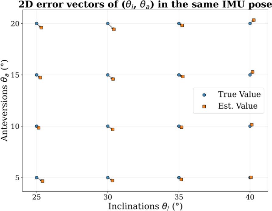
This experiment is divided into two parts. In the proposed method, when mounting the IMU onto the acetabular cup impactor, it is only required that its zI-axis is parallel to the acetabular cup axis. The first part of this experiment was to verify this claim. We selected two specific acetabular cup orientations — (θi,θa) = (25°,10°) and (35°,20°) — for testing. During the tests, the IMU’s pose was changed by rotating the circular turntable at the top of the tilt table, with the direction of the IMU zI-axis unchanged. The estimated results and the error vectors were recorded to analyze the influence of the IMU’s pose, as shown in Fig. 8. The results showed that the average magnitude of the error vectors was 0.987°, which increased compared to that before the IMU pose change (possibly due to jitter generated when rotating the turntable), but still remained within the tolerance range, indicating the method remains effective.
Comparison of error vectors in different IMU poses.
Due to the IMU drift error, which accumulates over time, the method proposed in this paper may become less effective over long-term use. Therefore, the second part of this experiment was designed to test the impact of the IMU drift. Similar to Experiment 3, the IMU measured θi and θa at a series of preset acetabular cup angles, with its pose unchanged. The difference in this experiment was that the procedure was conducted again after 10 and 20 minutes. The influence of drift was analyzed by comparing the error vectors of the estimated values at different times (as shown in Fig. 9).
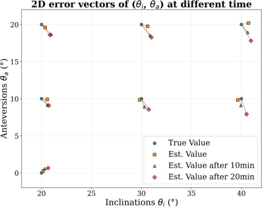
Comparison of error vectors at different times.
The RMSE of measurements and the average magnitude of error vectors at different times are listed in Table 5. Obviously, the IMU drift affected measurement accuracy, as all error results increased progressively with the extension of the test duration. However, even when the test was conducted after 20 minutes, the average error increased approximately 3.5 times, and the absolute errors remained within ±3°, largely meeting the accuracy requirements for acetabular cup orientation measurement. Considering that the acetabular cup implantation procedure in surgery takes approximately 30 minutes, it is recommended that surgeons perform secondary registration midway through the operation to recalibrate the IMU’s angle measurements.
Results of θi and θa measurement accuracy experiment.
| Test time | θi RMSE | θa RMSE | Average error vector magnitude |
|---|---|---|---|
| 0 min | 0.469° | 0.234° | 0.494° |
| 10 min | 0.618° | 1.085° | 1.199° |
| 20 min | 0.791° | 1.586° | 1.704° |
This work shows advantages across multiple aspects, including high prosthesis compatibility, non-invasiveness, and no radiation exposure when compared with other existing technologies, as presented in Table 6. In particular, its angular measurement error is significantly lower than that of other technologies. However, it must be noted that this excellent angular measurement accuracy is associated with the experimental environment. This work was tested on a precise 3-axis tilt table, which eliminated errors caused by patient position shifts and human soft tissue compression. Therefore, the previously mentioned experiments primarily verified the theoretical correctness and feasibility of the proposed method under ideal conditions. Meanwhile, it also indicates that this work needs to be further validated through in vitro tests and clinical trials in the future to examine its effectiveness in complex real surgical scenarios.
Performance comparison among different prosthesis pose estimation technologies for THA.
| This work | Chen et al. (2021) [16] | Tang et al. (2025) [17] | Computer-assisted system [11] | |
|---|---|---|---|---|
| Sensor type | IMU | IMU | IMU | camera |
| Angular error | RMSE: | RMSE: | MAE: | MAE: |
| Prosthesis adaptability | high | low | low | high |
| Invasiveness | non-invasive | non-invasive | non-invasive | invasive |
| Radiation exposure | no | no | no | yes |
| Experimental environment | 3-axis tilt table | customized measuring device | in vitro tests on sawbones | real cases (25 patients) |
This paper presents an intraoperative method for measuring acetabular cup inclination and anteversion in THA using an IMU, aiming to assist surgeons in implanting the cup within the "safe zone" (inclination: 40°±10°, anteversion: 15°±10°). Compared to traditional techniques, the method offers distinct benefits: real-time measurement, high accuracy, radiation-free operation, cost-effectiveness, non-invasiveness, and independence from bony landmarks.
Four experiments using a 3-axis tilt table evaluated its performance. The IMU’s reliability was validated with pose estimation RMSE ranging from 0.315° to 0.423°. The rotation axis vector for registration could be accurately acquired, with slight variations from IMU pose and rotation angle. Another test demonstrated high accuracy in measuring cup orientations (RMSE: 0.278° for inclination, 0.296° for anteversion; average error vector: 0.373°), well within clinical tolerance. Robustness tests showed that the IMU drift caused errors to increase approximately 3.5 times after 20 minutes. To address this, re-registration is recommended every 15 minutes to reduce drift errors.
The method’s feasibility was verified through theoretical derivation and experiments. However, the method relies on the assumption of relative immobility between the patient and the operating table, and the mid-procedure re-registration for drift mitigation adds modest operational complexity. Additionally, clinical trials are needed to verify its medical effectiveness. To address these limitations, future research will focus on conducting prospective clinical trials to quantify the effects of soft tissue compression and on optimizing data fusion algorithms to enhance drift suppression. With further optimization, the method has the potential to become a standard navigation method for THA.