
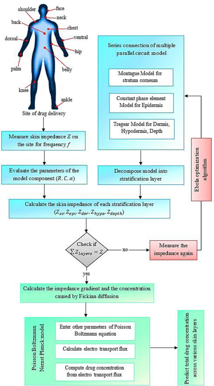
Fig. 1.
Sequence of steps adopted in this research for drug delivery.
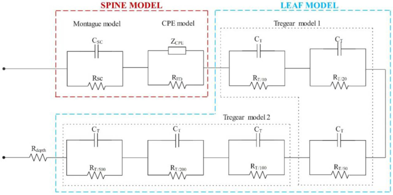
Fig. 2.
Spine–leaf resistor–capacitor circuit.
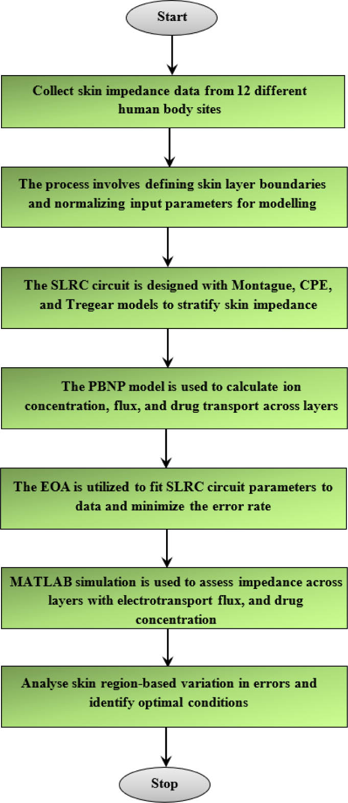
Fig. 3.
Flowchart of the proposed model for predicting drug penetration across various skin layers.
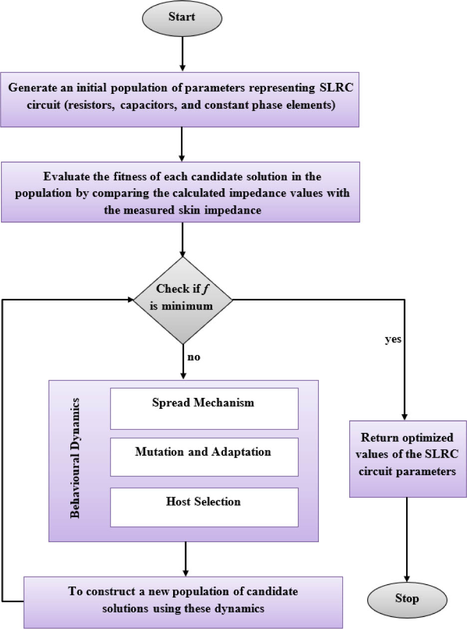
Fig. 4.
Flowchart of the Ebola Optimisation Algorithm for SLRC circuit parameter normalisation.
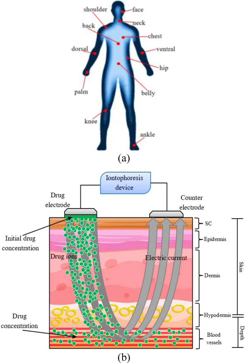
Fig. 5.
Visual representation of (a) Anatomical sites on the human body considered for iontophoretic drug delivery simulation. (b) Simulated drug concentration profiles across skin depths using the proposed model.
Table 1.
Impedance [Ω cm2] across different skin layers for all models.
| Layer | Montague | CPE | Tregear-1 | Tregear-2 | SLRC (proposed) |
|---|---|---|---|---|---|
| SC | 8452.34 | 8339.12 | 8210.89 | 6543.78 | 6520.43 |
| Epidermis | 6295.12 | 6203.98 | 6289.67 | 5082.34 | 4752.89 |
| Dermis | 783.12 | 710.45 | 735.56 | 850.92 | 903.78 |
| Hypodermis | 365.45 | 285.67 | 299.45 | 522.34 | 610.12 |
| Depth | 8.21 | 0.12 | 0.00 | 276.45 | 371.54 |
Table 2.
Electrotransport flux [μg/mm2s] across different skin layers for all models.
| Layer | Montague | CPE | Tregear-1 | Tregear-2 | SLRC (proposed) |
|---|---|---|---|---|---|
| SC | 167.12 | 162.34 | 165.45 | 139.87 | 126.78 |
| Epidermis | 125.87 | 122.76 | 123.56 | 103.45 | 95.34 |
| Dermis | 17.12 | 15.78 | 16.45 | 18.12 | 17.89 |
| Hypodermis | 7.12 | 6.45 | 6.89 | 11.34 | 13.56 |
| Depth | 0.34 | 0.00 | 0.12 | 5.87 | 7.34 |
Table 3.
Total drug concentration [mole/m3] across different skin layers for all models.
| Layer | Montague | CPE | Tregear-1 | Tregear-2 | SLRC (proposed) |
|---|---|---|---|---|---|
| SC | 390.67 | 387.12 | 392.34 | 418.12 | 378.56 |
| Epidermis | 328.45 | 324.67 | 326.12 | 275.67 | 260.78 |
| Dermis | 7.12 | 6.89 | 7.34 | 6.12 | 7.45 |
| Hypodermis | 3.89 | 2.87 | 3.23 | 4.45 | 5.34 |
| Depth | 0.65 | 0.00 | 0.12 | 1.78 | 2.56 |
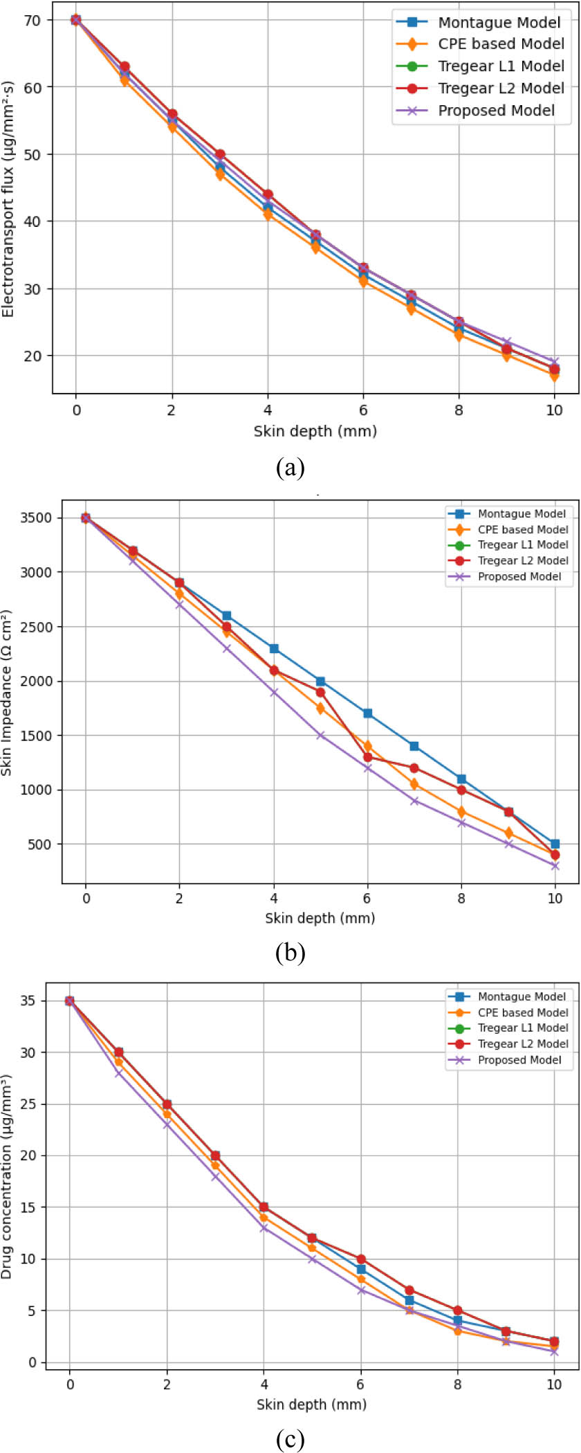
Fig. 6
(a) Skin impedance; (b) Electrotransport flux; and (c) Drug concentration derived from the electrotransport component with variation in skin depth.
Table 4.
Total drug concentration [mole/m3] with variations in current density (I, mA/cm2).
| I [mA/cm2] | I = 0.1 | I = 0.2 | I = 0.4 | I = 0.5 | I = 1.0 |
|---|---|---|---|---|---|
| SC | 140.12 | 205.36 | 329.85 | 392.47 | 710.29 |
| Epidermis | 89.34 | 132.19 | 218.76 | 261.42 | 480.14 |
| Dermis | 2.32 | 3.76 | 6.45 | 7.84 | 15.08 |
| Hypodermis | 1.63 | 2.42 | 3.89 | 4.51 | 8.12 |
| Depth | 1.24 | 1.62 | 2.36 | 2.72 | 4.51 |
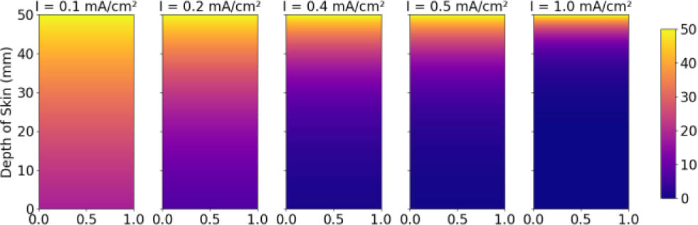
Fig. 7.
Total drug concentration [μg/mm3] at different skin layers in current density [mA/cm2].
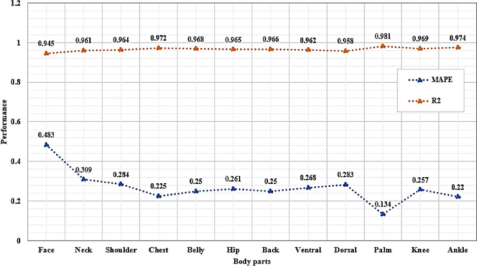
Fig. 8.
Analysis of the proposed model based on MAPE and R2 values across various body regions.
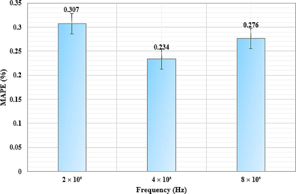
Fig. 9.
Performance analysis of the proposed model based on MAPE vs Frequency for TDD.
Table 5.
Mean and SD [Ω] of impedance for various body parts.
| Body parts | 2 × 10³ Hz | 4 × 10³ Hz | 8 × 10³ Hz | |||
|---|---|---|---|---|---|---|
| Mean | SD | Mean | SD | Mean | SD | |
| Face | 5.60 × 10³ | 1840.12 | 4.20 × 10³ | 1450.25 | 6.80 × 10³ | 2115.37 |
| Neck | 1.02 × 10⁴ | 2155.20 | 7.85 × 10³ | 1780.55 | 1.12 × 10⁴ | 2401.28 |
| Shoulder | 1.10 × 10⁴ | 2250.30 | 8.20 × 10³ | 1720.45 | 1.18 × 10⁴ | 2435.12 |
| Chest | 1.25 × 10⁴ | 2445.41 | 9.05 × 10³ | 1865.33 | 1.34 × 10⁴ | 2560.11 |
| Belly | 1.30 × 10⁴ | 2235.75 | 9.50 × 10³ | 1900.25 | 1.38 × 10⁴ | 2710.32 |
| Hip | 1.18 × 10⁴ | 2145.88 | 8.70 × 10³ | 1805.40 | 1.26 × 10⁴ | 2605.45 |
| Back | 1.12 × 10⁴ | 2140.82 | 8.50 × 10³ | 1775.55 | 1.22 × 10⁴ | 2525.87 |
| Ventral | 1.25 × 10⁴ | 2195.65 | 9.20 × 10³ | 1825.75 | 1.32 × 10⁴ | 2650.20 |
| Dorsal | 1.50 × 10⁴ | 2280.34 | 1.05 × 10⁴ | 1950.45 | 1.60 × 10⁴ | 2755.30 |
| Palm | 1.75 × 10⁴ | 2370.12 | 1.20 × 10⁴ | 2050.50 | 1.85 × 10⁴ | 2855.20 |
| Knee | 1.45 × 10⁴ | 2200.55 | 1.00 × 10⁴ | 1850.15 | 1.55 × 10⁴ | 2705.75 |
| Ankle | 1.60 × 10⁴ | 2335.22 | 1.12 × 10⁴ | 1955.40 | 1.70 × 10⁴ | 2800.35 |
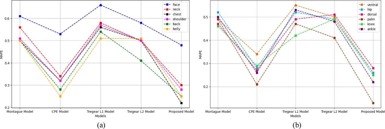
Fig. 10.
MAPE value comparison of different models for different body parts (a) Upper body regions and (b) Lower body regions.
Table 6.
Comparison analysis of the proposed SLRC circuit with existing models across various body parts.
| MAPE values | Rsc | CT | SF | R2 | |||||
|---|---|---|---|---|---|---|---|---|---|
| Body parts | Montague | CPE | Tregear-1 | Tregear-2 | Proposed | Proposed | Proposed | Proposed | Proposed |
| Face | 0.613 | 0.531 | 0.665 | 0.582 | 0.483 | 72.476 | 0.495 | 1.000 | 0.945 |
| Neck | 0.561 | 0.342 | 0.585 | 0.506 | 0.309 | 17.465 | 0.496 | 0.924 | 0.961 |
| Shoulder | 0.518 | 0.320 | 0.578 | 0.501 | 0.284 | 13.584 | 0.451 | 0.870 | 0.964 |
| Chest | 0.501 | 0.320 | 0.564 | 0.507 | 0.225 | 10.027 | 0.447 | 0.884 | 0.972 |
| Belly | 0.505 | 0.256 | 0.515 | 0.519 | 0.250 | 45.268 | 0.312 | 0.998 | 0.968 |
| Hip | 0.520 | 0.280 | 0.528 | 0.498 | 0.261 | 38.923 | 0.315 | 0.962 | 0.965 |
| Back | 0.505 | 0.284 | 0.546 | 0.415 | 0.250 | 15.385 | 0.286 | 0.984 | 0.966 |
| Ventral | 0.494 | 0.343 | 0.556 | 0.506 | 0.268 | 23.948 | 0.471 | 0.908 | 0.962 |
| Dorsal | 0.475 | 0.272 | 0.495 | 0.512 | 0.283 | 80.638 | 0.352 | 1.000 | 0.958 |
| Palm | 0.494 | 0.211 | 0.472 | 0.418 | 0.134 | 18.225 | 0.441 | 0.844 | 0.981 |
| Knee | 0.463 | 0.297 | 0.424 | 0.495 | 0.257 | 55.687 | 0.346 | 0.975 | 0.969 |
| Ankle | 0.505 | 0.266 | 0.532 | 0.483 | 0.220 | 40.315 | 0.417 | 0.903 | 0.974 |