
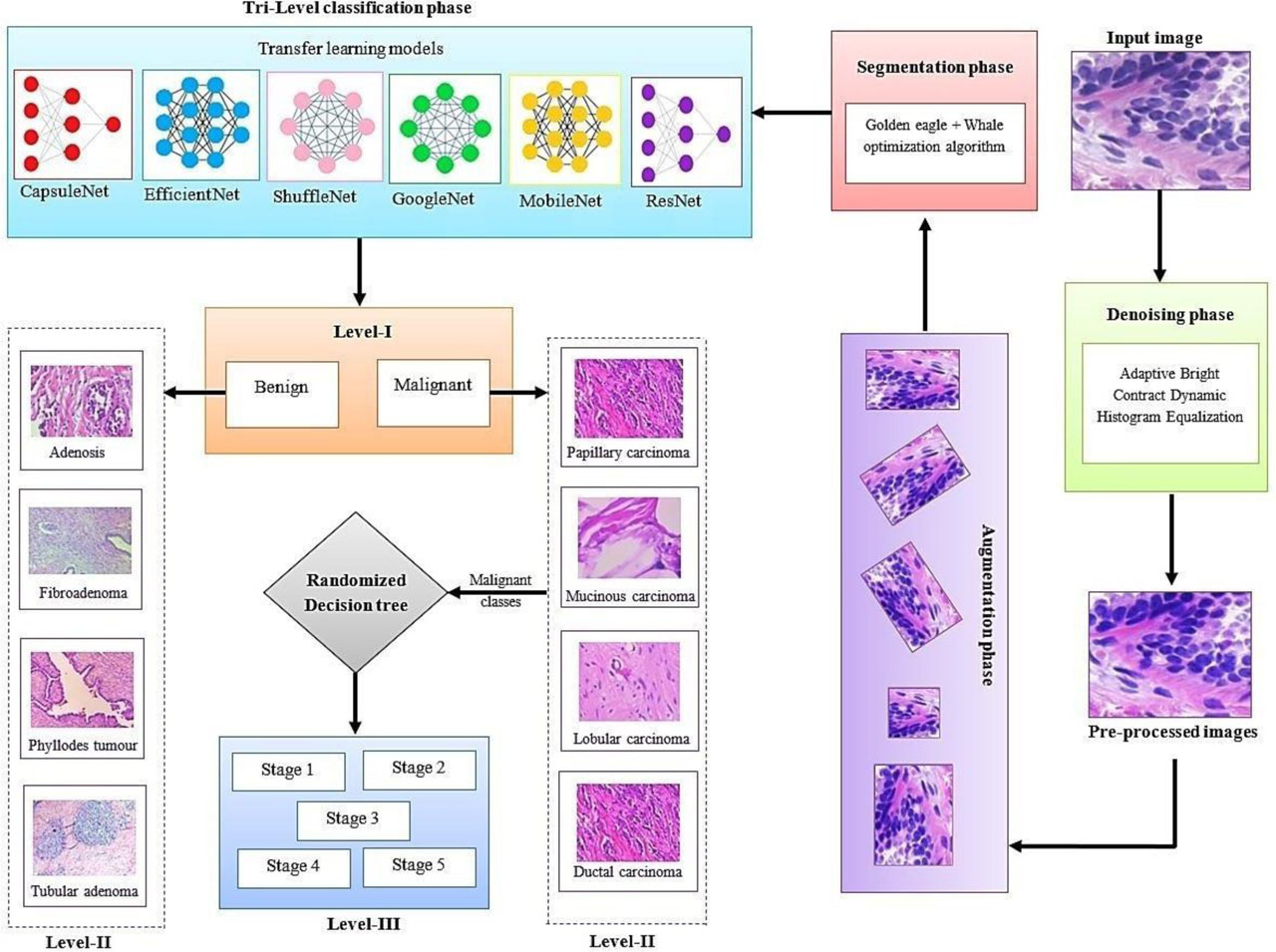
Fig. 1.
Schematic illustration of the proposed TRI-BCC model.
Table 1.
Dataset description of BreakHis with image count.
| Class type | Subtype | Image count |
|---|---|---|
| Benign | AS | 444 |
| FA | 1442 | |
| PT | 209 | |
| TA | 385 | |
| Malignant | DC | 3450 |
| LC | 626 | |
| MC | 792 | |
| PC | 561 | |
| Total | 7909 |
Table 2.
Stage-wise distribution of malignant subtypes.
| Malignant subtype | Stage 1 | Stage 2 | Stage 3 | Stage 4 | Stage 5 | Total |
|---|---|---|---|---|---|---|
| DC | 460 | 790 | 970 | 670 | 560 | 3450 |
| LC | 110 | 160 | 140 | 110 | 106 | 626 |
| MC | 160 | 205 | 190 | 125 | 112 | 792 |
| PC | 105 | 130 | 145 | 90 | 91 | 561 |
| Total | 835 | 1285 | 1445 | 995 | 869 | 5429 |
Table 3.
Augmentation count after targeted augmentation techniques.
| Class type | Subtype | Original count | Augmented count | Total count |
|---|---|---|---|---|
| Benign | AS | 444 | 400 | 844 |
| FA | 1442 | 0 | 1442 | |
| PT | 209 | 500 | 709 | |
| TA | 385 | 300 | 685 | |
| Subtotal | 2480 | 1200 | 3680 | |
| Malignant | DC | 3450 | 0 | 3450 |
| LC | 626 | 0 | 626 | |
| MC | 792 | 0 | 792 | |
| PC | 561 | 0 | 561 | |
| Subtotal | 5429 | 0 | 5429 | |
| Total | 7909 | 0 | 9109 |
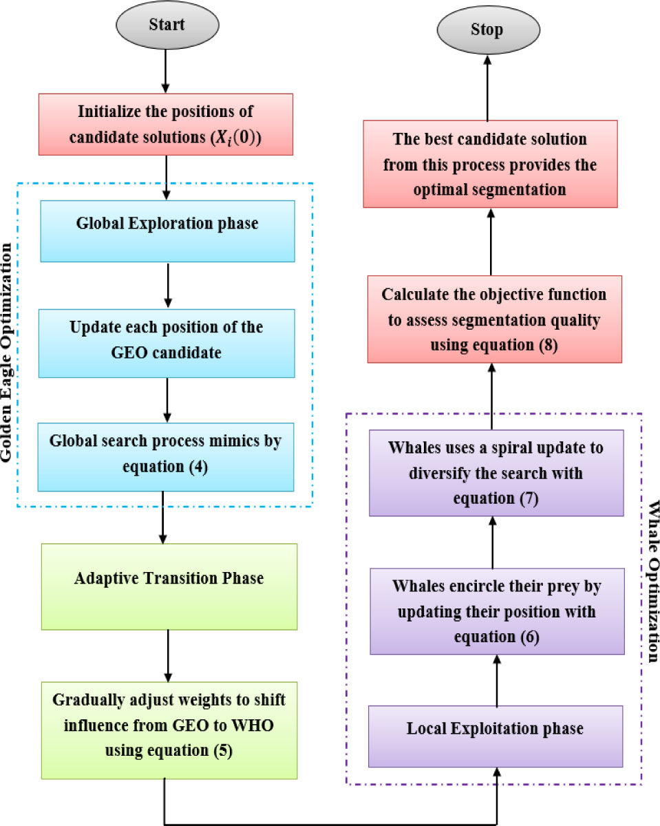
Fig. 2.
Flowchart of the proposed GWO algorithm.
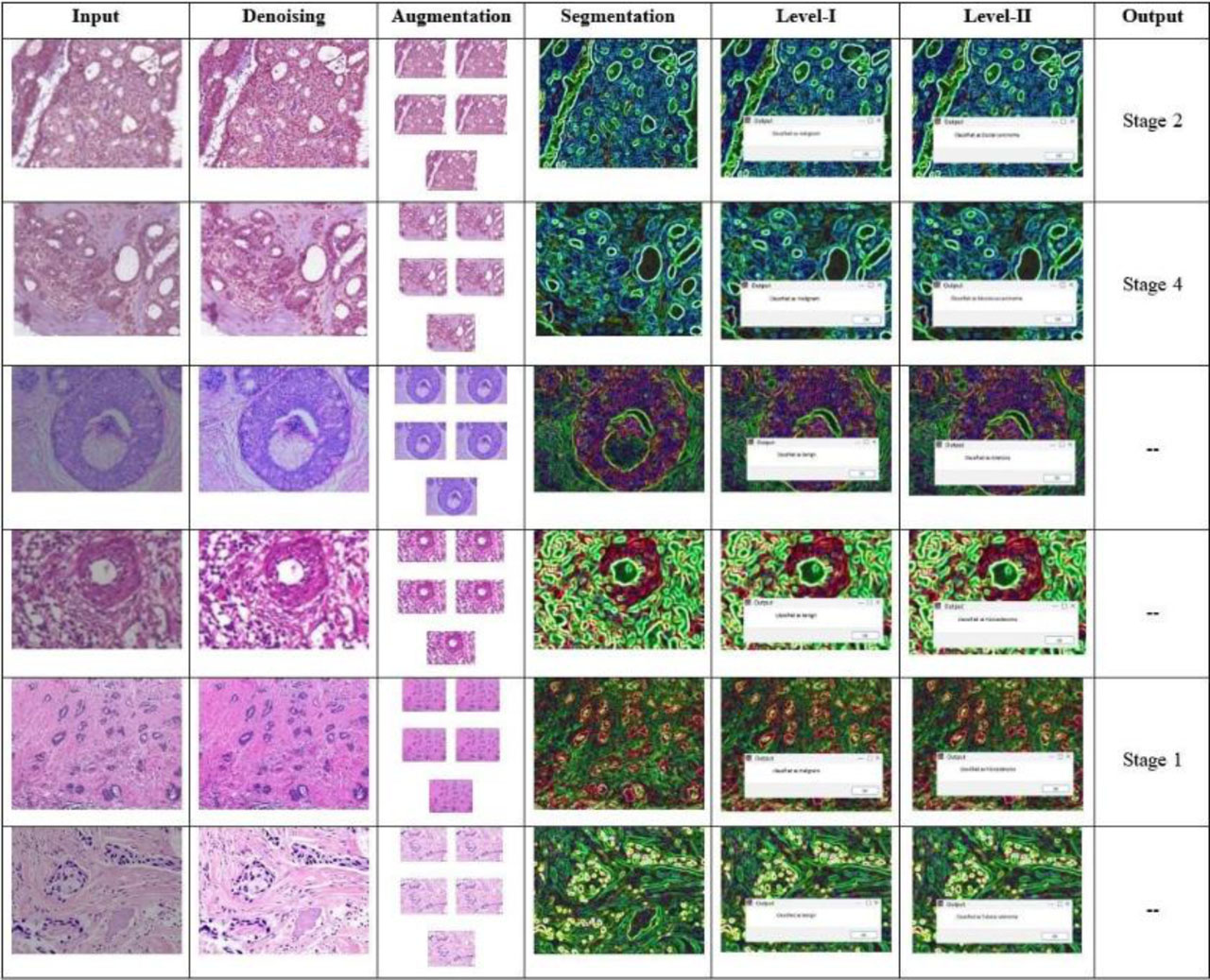
Fig. 3.
Experimental results of the proposed TRI-BCC model for BC classification.
Table 4.
Efficiency analysis of the proposed TRI-BCC model for Level-I.
| Classes | ACC | SPE | SEN | PRE | F1S |
|---|---|---|---|---|---|
| Benign | 99.25 | 99.01 | 98.73 | 98.45 | 98.18 |
| Malignant | 98.84 | 98.06 | 99.01 | 99.27 | 99.49 |
| Average | 99.04 | 98.95 | 98.69 | 99.49 | 98.47 |
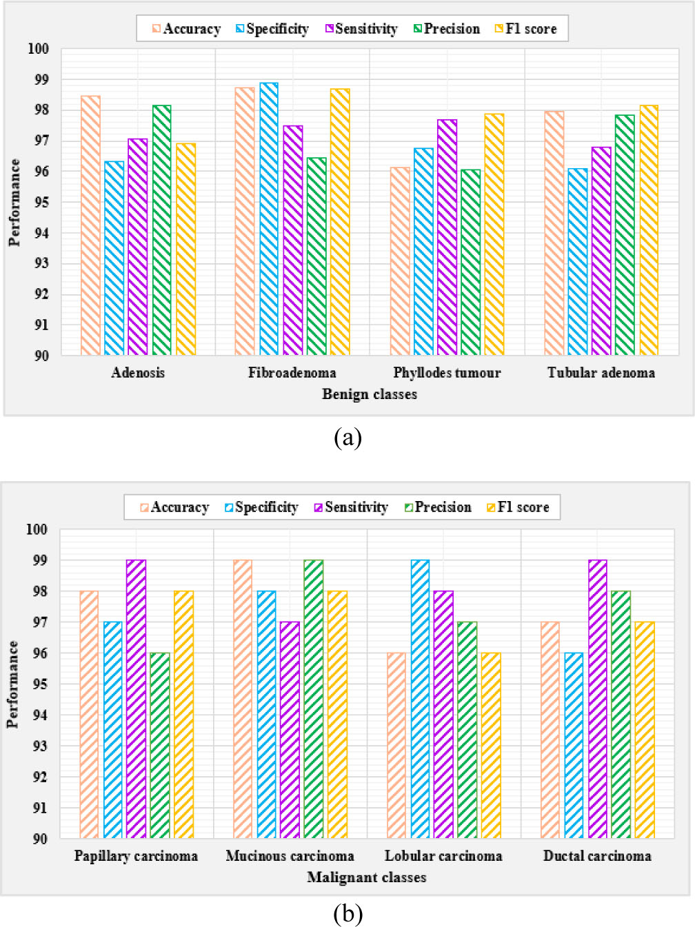
Fig. 4.
Level-II analysis of the proposed TRI-BCC model for (a) Benign classes and (b) Malignant classes.
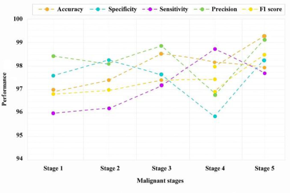
Fig 5.
Level-III analysis of the proposed TRI-BCC model for Malignant class stages.
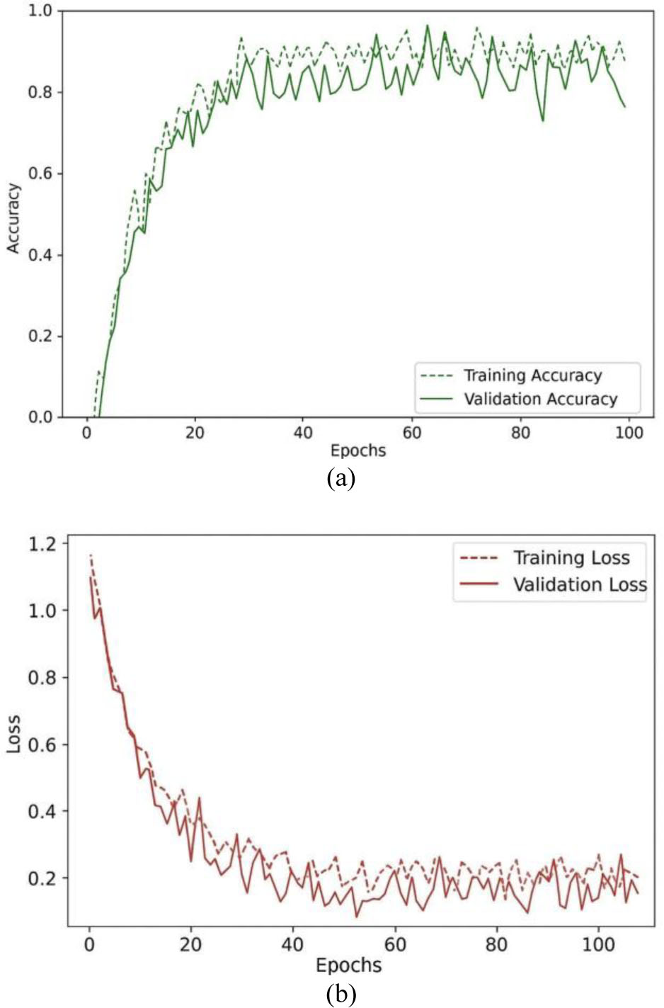
Fig. 6.
Training and testing curve of the proposed TRI-BCC model (a) Accuracy curve; (b) Loss curve.
Table 6.
Comparative evaluation of different ML classification models.
| Methods | ACC | SPE | SEN | PRE | F1S |
|---|---|---|---|---|---|
| NB | 87.9 | 86.8 | 88.4 | 86.3 | 87.2 |
| DT | 94.7 | 94.0 | 95.5 | 93.1 | 94.2 |
| RF | 96.3 | 95.9 | 96.8 | 95.4 | 96.1 |
| KNN | 89.5 | 89.0 | 90.2 | 88.7 | 89.1 |
| RDT | 99.04 | 98.9 | 98.6 | 99.4 | 98.4 |
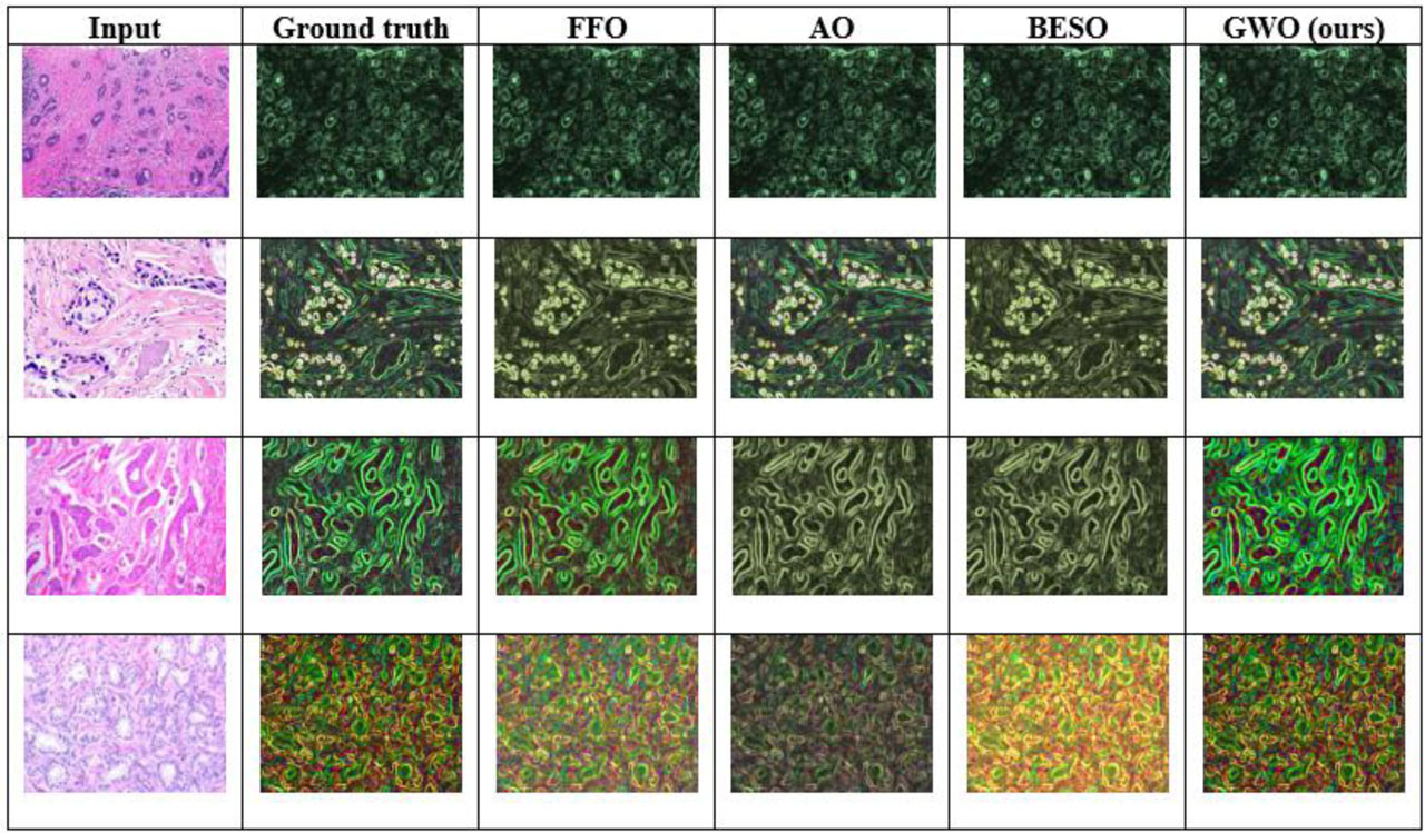
Fig. 7.
Visual comparison of different optimization algorithms for segmentation.