
Table 1.
Literature review.
| Author | Method | Outcome | Advantages | Drawbacks |
|---|---|---|---|---|
| Arun and Sahaya Aarti [21] | MPC | Rise time is 262 s, overshoot is 9.3 % | Lower peak and settling time | Overshoot is higher in the second tank |
| Kumar et al. [22] | IMC-PID | ITAE is 0.0661, overshoot is 7.611·10-4 | It can be applied to the conical transfer function | Poor robustness |
| Rajiv Ranjan [23] | MRAC | Settling time is 30 s | System performance is stable under unmodelled dynamic | Longer settling time |
| Espitia-Cuchango et al. [24] | NFAC | Desired response is obtained under varying system conditions | Suitable for multi-input and multi-output systems | More settling time |
| Aguila-Camacho et al. [25] | FOPI | ITAE is 1.4465·106 | Lower variance | More time to settle |
| Balaska et al. [29] | FO-MRAC | Sampling period is 0.1 s | Lowest error cost | Increases the noise |
| Patil and Agashe [30] | DRL | Desired response is obtained under varying system conditions | Reduces the complexity and non-linearity | Higher rise time |
| Ramanathan et al. [31] | Reinforcement learning algorithm | Settling time for trial 1 is 452 s | Reduces the non-linearity issues and settling time | Learning process slow |
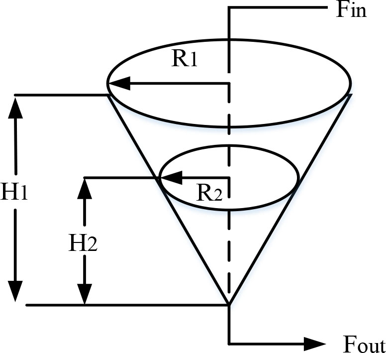
Fig. 1.
Structure of a CT.
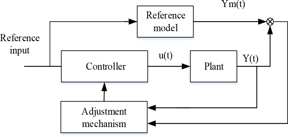
Fig. 2.
Block diagram of MRAC.
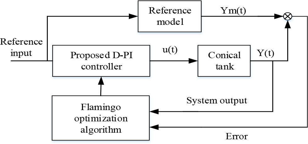
Fig. 3.
Proposed MRAC with D-PI.
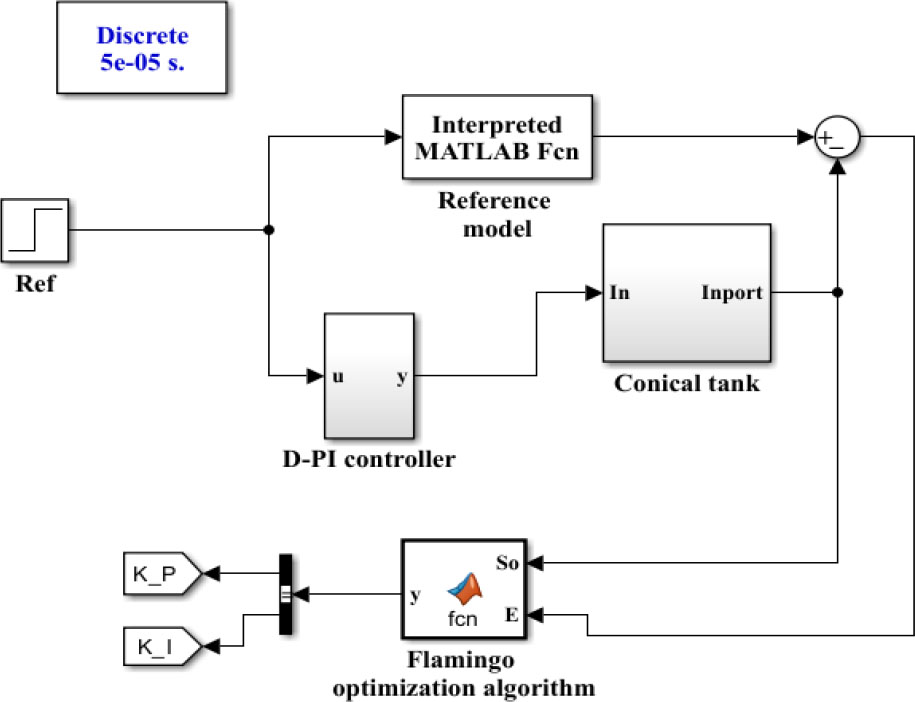
Fig. 4.
Simulink model of MRAC with CT.
Table 2.
Comparative analysis of different controllers.
| Controllers | Peak overshoot [%] | Settling time [s] | Rise time [s] | ISE | IAE |
|---|---|---|---|---|---|
| PI | 18.17 | 402 | 109 | 47.73 | 2681 |
| PID | 21.32 | 421 | 114 | 51.03 | 2968 |
| FOPI | 12.74 | 408 | 157 | 43.09 | 2902 |
| MRAC-PID | 7.19 | 391 | 174 | 41.35 | 2863 |
| MRAC (Proposed) | 0.8 | 200 | 103 | 38.25 | 2167 |
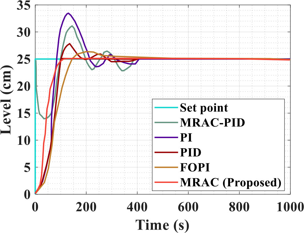
Fig. 5.
Controller output under constant set point.
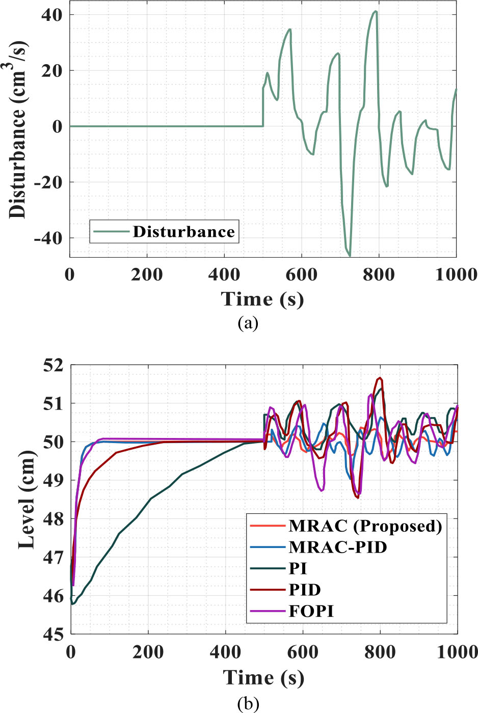
Fig. 6.
Performance analysis under random disturbance in constant setpoint.
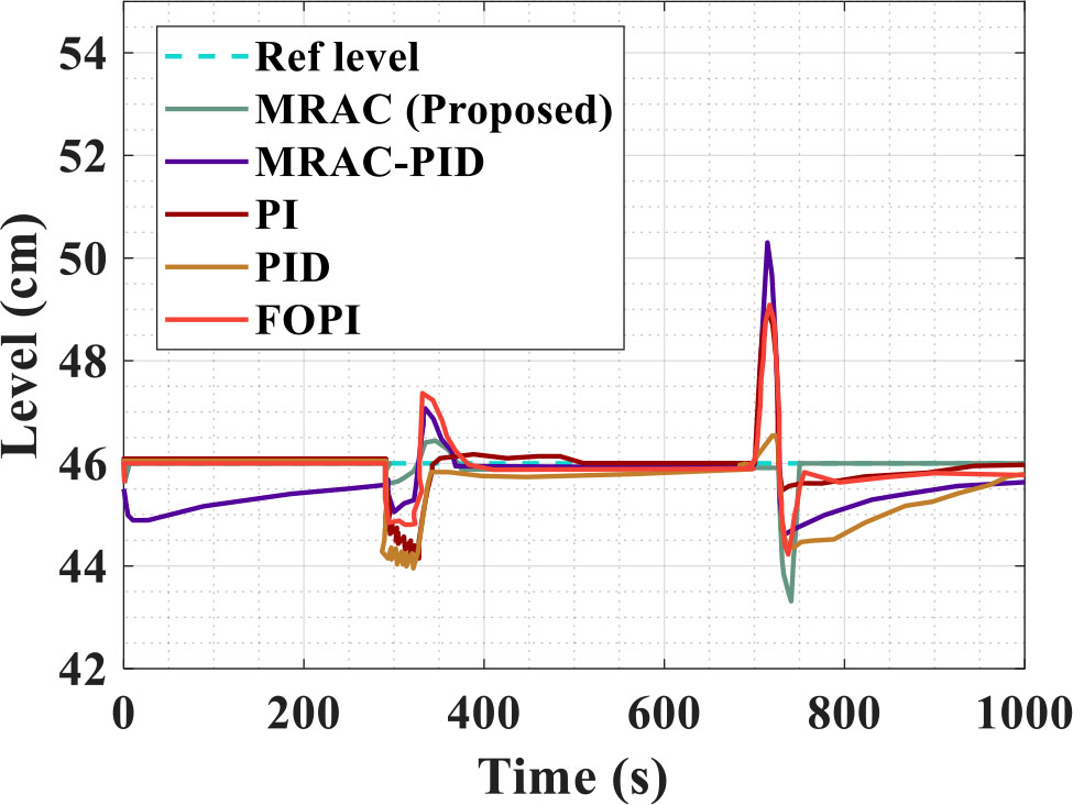
Fig. 7.
Performance analysis under load variations.
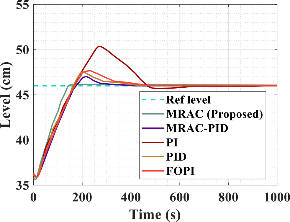
Fig. 8.
Controller output under variation in reference from 30 cm to 46 cm.
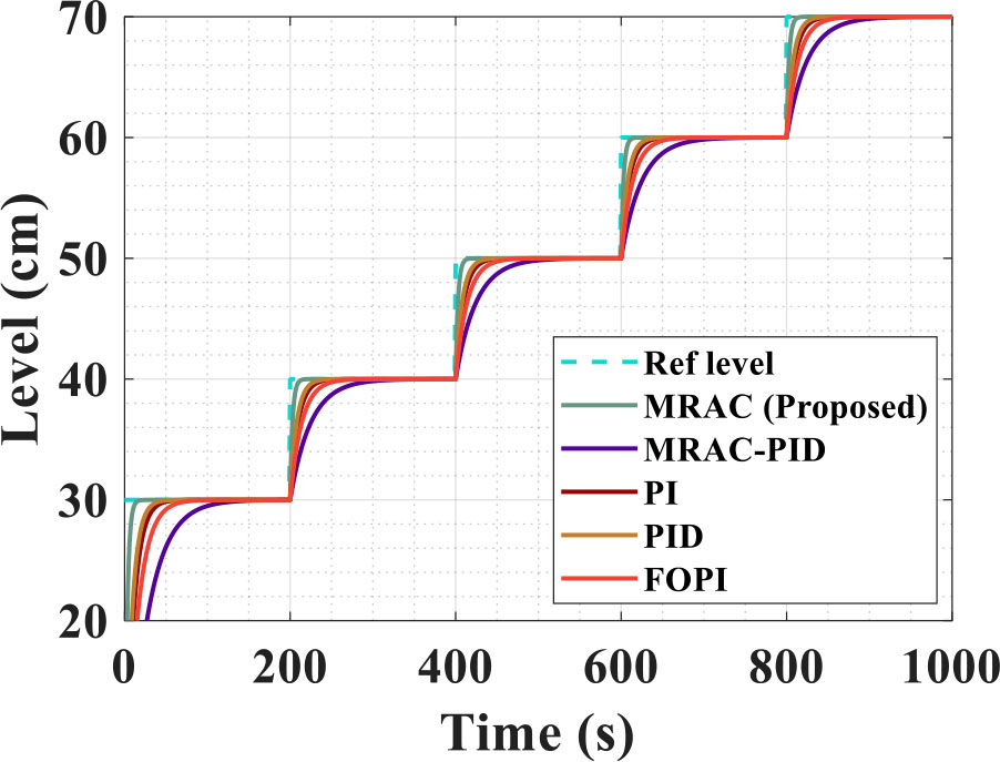
Fig. 9.
Controller response under varying liquid levels.
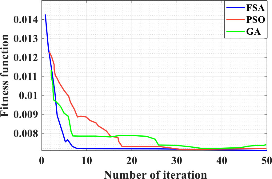
Fig. 10.
Convergence plot for optimization algorithms.
Table 3.
Comparative analysis of PID controller with different optimization techniques.
| Controllers | Peak overshoot [%] | Settling time [s] | Rise time [s] | ISE | IAE |
|---|---|---|---|---|---|
| PID | 21.32 | 421 | 114 | 51.03 | 2968 |
| PID with GA | 10.52 | 376 | 131 | 44.17 | 2888 |
| PID with PSO | 5.44 | 305 | 122 | 40.93 | 2652 |
| MRAC (Proposed) | 0.8 | 200 | 103 | 38.25 | 2167 |
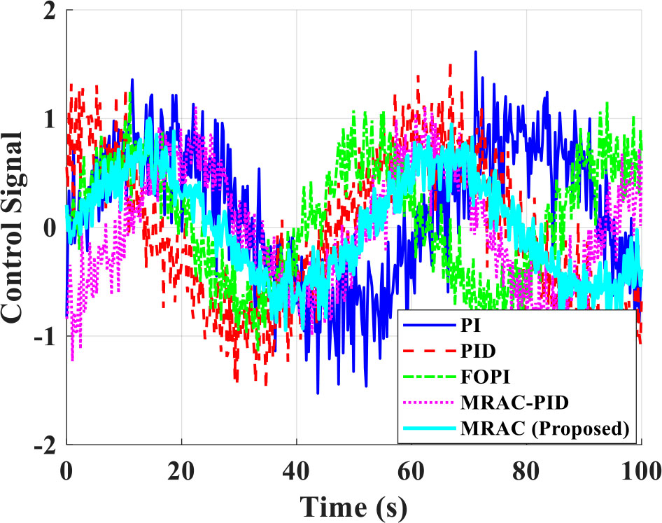
Fig. 11.
Comparison of control signals for different controllers.