
Table 1.
Hybrid ML models.
| Applied ML model | Research description |
|---|---|
| SVM with GA | A study applied SVM combined with GA to develop optimal classifiers for distinguishing healthy and faulty bearings in ASD systems, achieving 97.5 % accuracy [21]. |
| SVM and ANN with CWT | This study explored the use of SVM and ANN alongside CWT to analyze frame vibrations during motor start-up, achieving 96.67 % accuracy with SVM and 90 % with ANN [22]. |
| PCA and SVDD | PCA and SVDD were used to predict bearing failures, achieving 93.45 % accuracy [23]. |
| GA-based SVM | A GA-based kernel discriminative feature analysis was combined with one-against-all multicategory SVMs (OAA MCSVMs) for fault diagnosis in low-speed bearings, achieving the highest reported accuracy of 98.66 % [24]. |
| FEM and WPT with SVM | A hybrid approach integrating FEM, WPT, and SVM was proposed for fault classification, achieving 81 % accuracy for inner race faults and 79 % for rolling body faults [25]. |
| FFT-based feature extraction with SVM | The frequency domain features derived from FFT were used to train an SVM model for bearing fault classification, achieving 87.35 % accuracy [26]. |
[i] Note:
SVM - support vector machines
GA - genetic algorithm
ASD - adjustable speed drive
ANN - artificial neural networks
CWT - continuous wavelet transform
PCA - principal component analysis
SVDD - support vector data description
FEM - finite element method
OAA - one-against-all
MCSVM - multicategory SVM
WPT - wavelet packet transform
FFT - fast fourier transform
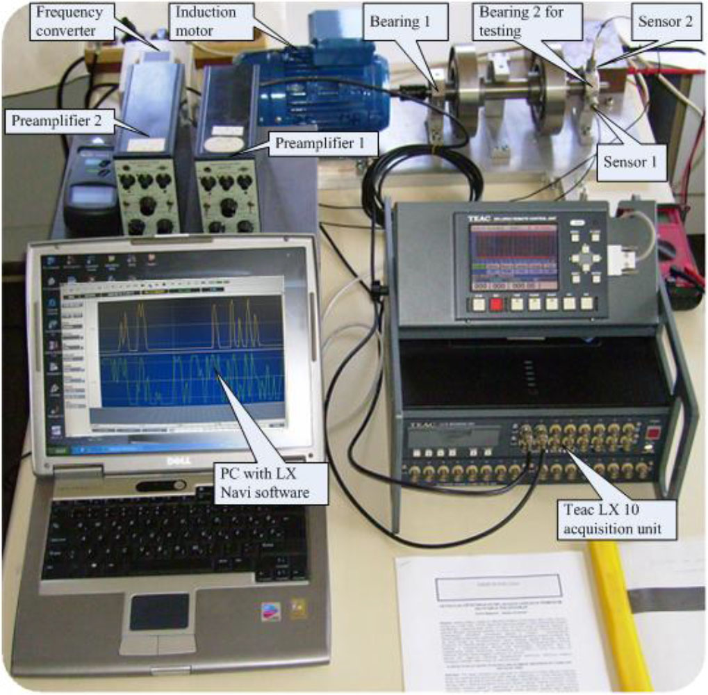
Fig. 1.
The developed ball bearing test station.
Table 2.
The k-nearest neighbor (KNN) classification.
| Model No | Model name | Distance metric | Distance weight | Number of neighbors | Classification success rate |
|---|---|---|---|---|---|
| 1 | Cosine KNN | Cosine | Equal | 10 | 98.5 % |
| 2 | Coarse KNN | Euclidean | Equal | 100 | 74 % |
| 3 | Fine KNN | Euclidean | Equal | 1 | 97.4 % |
| 4 | Weighted KNN | Euclidean | Squared inverse | 10 | 97.4 % |
| 5 | Medium KNN | Euclidean | Equal | 1 | 98 % |
| 6 | Cubic KNN | Minkowski | Equal | 10 | 98.2 % |
Table 3.
SVM classification.
| Model No | Kernel function | Classification success rate |
|---|---|---|
| 1 | Linear | 93.9 % |
| 2 | Polynomial (ρ = 2) | 99.5 % |
| 3 | RBF | 99 % |
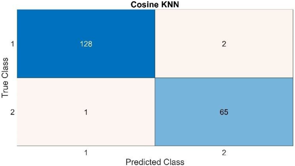
Fig. 2.
Confusion matrix for the cosine KNN algorithm.
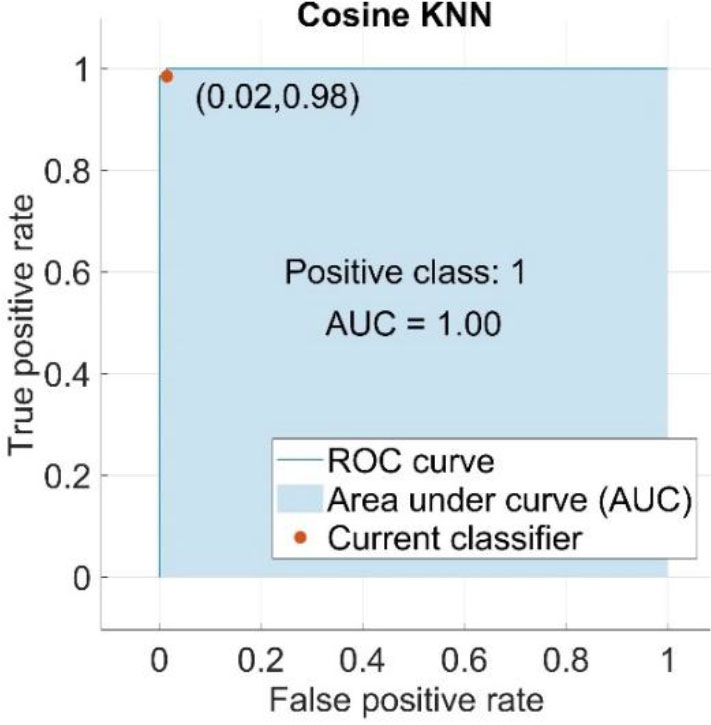
Fig. 3.
ROC curve for the cosine KNN algorithm.
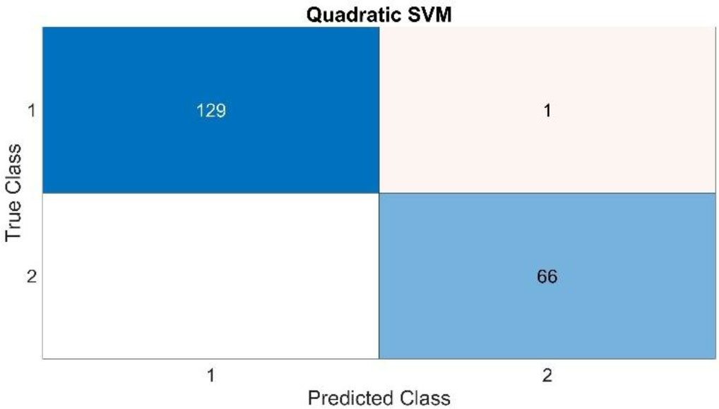
Fig. 4.
Confusion matrix for the quadratic SVM algorithm.
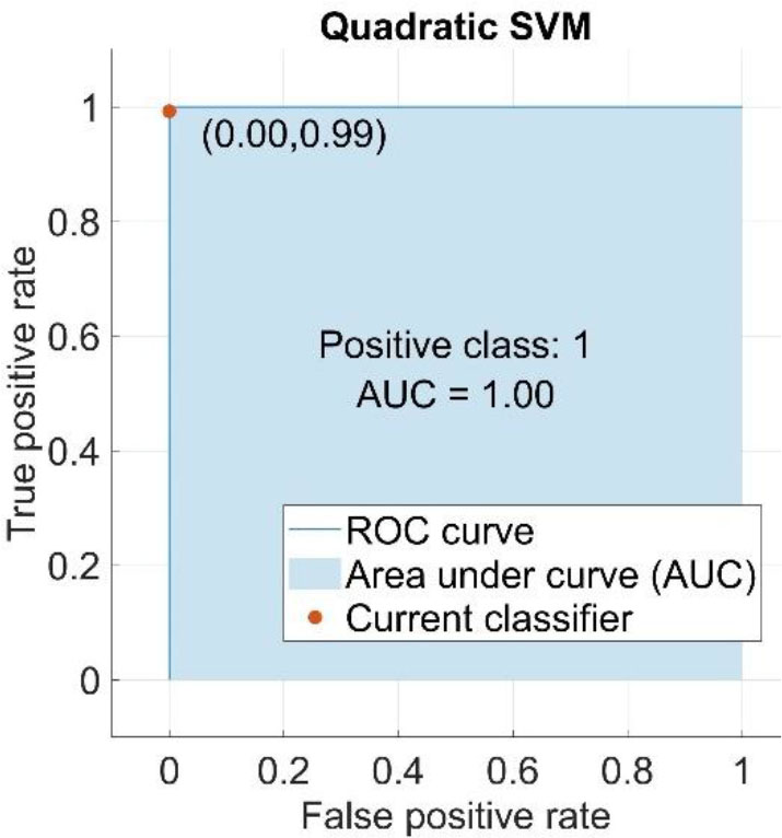
Fig. 5.
ROC curve for the quadratic SVM algorithm.
Table 4.
SVM hyperparameter search range.
| Hyperparameter | Range |
|---|---|
| Box constraint level | 0.001-1000 |
| Kernel scale | 0.001-1000 |
| Kernel function | Gaussian, Linear, Quadratic, Cubic |
| Standardize data | true, false |
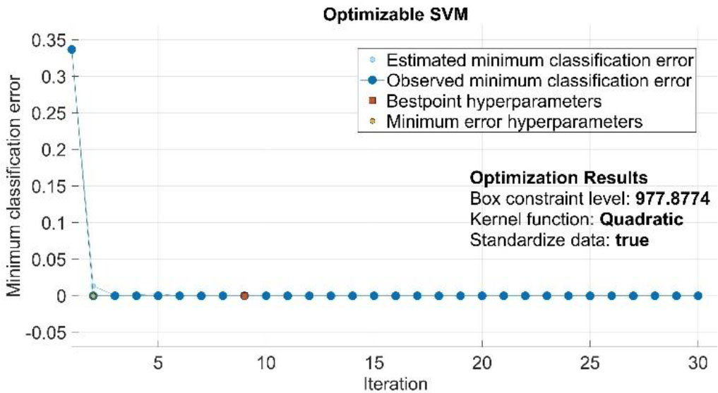
Fig. 6.
The optimization flow for the SVM algorithm.
Table 5.
The optimized hyperparameters of the SVM algorithm.
| Hyperparameter | Value |
|---|---|
| Box constraint level | 977.88 |
| Kernel scale | 1 |
| Kernel function | Quadratic |
| Standardize data | true |
| Accuracy | 100 % |
Table 6.
KNN hyperparameter search range.
| Hyperparameter | Range |
|---|---|
| Number of neighbors | 1–98 |
| Distance metric | Euclidean, Cosine, Euclidean, Correlation, Chebyshev, Hamming, Minakowski, Spearman, Jaccard, City block, Mahalanobis |
| Distance weight | Equal, Inverse, Squared, Inverse |
| Standardize data | true, false |
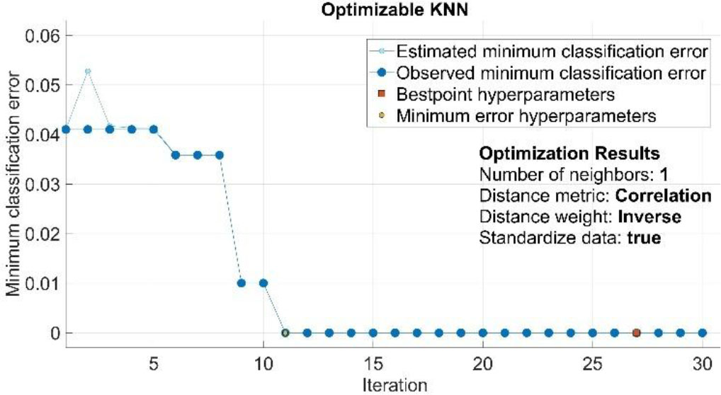
Fig. 7.
The optimization flow for the KNN algorithm.