
The variation in regulatory building provisions across different countries presents a significant challenge, particularly in adapting to these differences, which poses an additional hurdle for engineers. The building codes vary in terms of design equations, safety factors for materials, load considerations, etc. Understanding the key characteristics and distinctions among different building codes of practice is considered essential for establishing consistent guidelines worldwide. The concrete may not be able to achieve the necessary compression force to resist the specified bending moment if the beam cross-section is restricted due to architectural or other considerations. By adding reinforcement in the compression zone, a doubly reinforced beam is formed, which has both compression and tension reinforcement [1,2]. Figure 1 illustrates the stress and strain distributions of a doubly reinforced rectangular beam, utilizing the simplified stress block, as outlined in ACI 318 [3]. The application of strength design approaches that consider the entire strength capacity of the concrete on the compressive side has led to a significant decrease in the use of compression reinforcement. Space or aesthetic limitations may necessitate the use of beams with small dimensions, which in turn requires the inclusion of compression steel alongside tensile steel reinforcement [4,5]. The moment capacity of a beam with a maximum reinforcement ratio can be enhanced by incorporating reinforcement in both the tensile and compression zones, particularly when
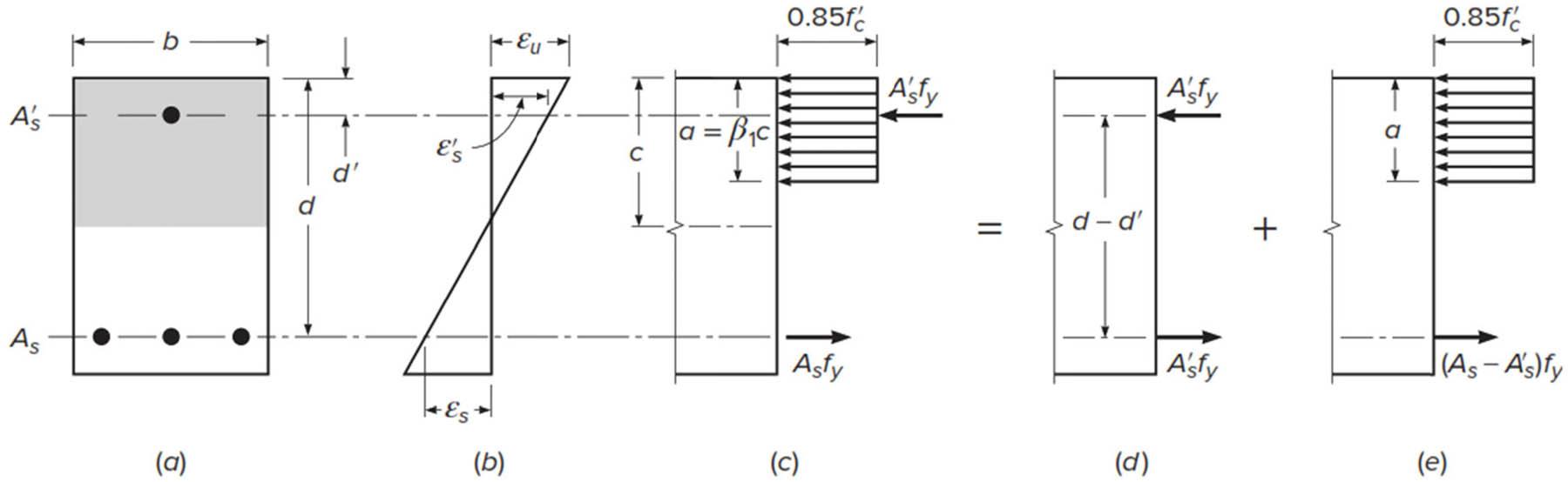
Analysis of a doubly reinforced rectangular beam [9]. (a) Cross-section, (b) Strain distribution, (c) Stress and forces, (d) Forces from Part 1, and (e) Forces from Part 2.
High-strength reinforcing steel had a characteristic yield strength of 500 MPa. This designation indicates that the steel has a minimum yield strength of 500 N/mm² under standard testing conditions. Grade 500 steel represents a higher strength classification compared to conventional reinforcing steel grades (such as Grade 240, Grade 360, or Grade 420), allowing for reduced cross-sectional areas of reinforcement while maintaining equivalent load-carrying capacity. The higher strength grade enables more economical designs and is particularly beneficial in high-rise construction and heavily loaded structural members where reinforcement congestion might otherwise be problematic. High-strength steel has been developed as a result of advancements in steel production, enabling the construction of thinner and more effective structural members. However, the behavior of such elements, especially shallow beams, requires further investigation to ensure their performance under various loading conditions [10,11]. The shallow beams can be defined as the structural members characterized by a span-to-depth ratio typically greater than 2.5–3.0, where the beam’s length significantly exceeds its cross-sectional depth. In shallow beams, plane sections remain approximately plane after bending (Bernoulli–Euler beam theory applies), and failure is generally governed by flexural behavior rather than shear. These beams exhibit linear strain distribution across their depth and are commonly found in typical building construction where architectural constraints limit beam depth. While the current design code (e.g., ACI 318 and EC 2) provides provisions for doubly reinforced shallow concrete beams, its adequacy with high-strength steel, such as grade 500 MPa and more, is inadequately verified. These codes were mainly developed and valid for members with normal-strength reinforcement. As a result, they may fail to make accurate predictions of the flexural capacity and failure mode of doubly reinforced shallow concrete beams, as they do not fully account for the beam failing before the maximum strain in the concrete on the compression side (0.003) associated with the high steel strength. This difference in code provisions requires targeted research to develop more reliable and efficient design models for this specific class of structural members. The primary possible failure of direct code application is threefold: (i) excessive crack width under service load – high-strength steel under service load at the same load level leads to proportionally wider flexural cracks compared to normal-strength steel. While codes such as ACI 318 provide cracked control equations, they are empirically derived from a database of beams with normal-strength steel. Their accuracy and safety when applied to beams made of high-strength steel, especially shallow beams where crack control is more critical, have not yet been fully verified. This can lead to non-compliance with states despite sufficient final strength, (ii) Deflection control – shallow beams are naturally susceptible to large deflection. The use of high-strength steel, with its highly acceptable stress, often results in small reinforcement areas (AS) for the same moment capacity. This reduces the stiffness of the section (effective moment of inertia, IE), possibly leading to deflections exceeding code-based boundaries, even if the needs of strength are satisfied. (iii) Ductility and minimum reinforcement requirements – code provisions for minimal flexural reinforcement (AS, min) are designed to ensure a ductile failure mode by giving steel yield before concrete crushing. These equations are a function of steel yield power (Fy). For high-strength steel, as min becomes quite small. In shallow beams, this minimum amount of steel may be insufficient to prevent a brittle failure or to control the cracks sufficiently, leading to a conflict between strength and serviceability design objectives.
In addition to strength, compressive reinforcement can be used for other reasons. The inclusion of compression steel has been observed as a factor in reducing the long-term deflections of flexural members. In certain instances, reinforcement bars will be positioned within the compression zone to accommodate minimal-moment loading conditions. Figure 2 illustrates an instance of the live load arrangement in the reinforced concrete frames. The objective of arranging live loads on reinforced concrete continuous beams is to identify the most important loading configurations that yield the maximum bending moments. The application of live load on some reinforced concrete beam spans generates negative moments in the unloaded spans, requiring the incorporation of steel in the compression zone to resist these moments.
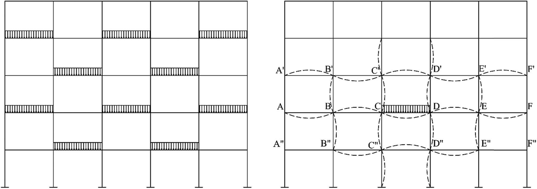
Alternate live loadings for minimum and maximum effects.
The compression zone will include bars as stirrup hangers that will remain throughout the beam span (as shown in Figure 3). When the longitudinal bars are cut off along the beam’s length due to reduced requirements for bending moment strength, a portion of the longitudinal bar must extend along the beam to function as stirrup hangers. Generally, building codes specify the required number of bars that must remain intact. The bars serving as stirrup hangers, typically located within the compression zone, are essential for the effective operation of shear reinforcement and the overall structural integrity of the reinforced concrete beam. They represent a crucial aspect in the realm of reinforced concrete construction. Although compression reinforcement is often neglected in flexural calculations, it may still be a good idea to take into account the presence of such reinforcement in flexural design. Therefore, this article aims to assess the validity of the accuracy analysis and design methods for doubly reinforced sections as suggested by various provisions and codes. The study conducted an experimental investigation that involved three beams, each with a compression steel to tension steel ratio of 0.2, 0.3, and 1. Furthermore, this study aims to develop a proposed analytical method for the design of doubly reinforced shallow beams utilizing grade 500 steel.
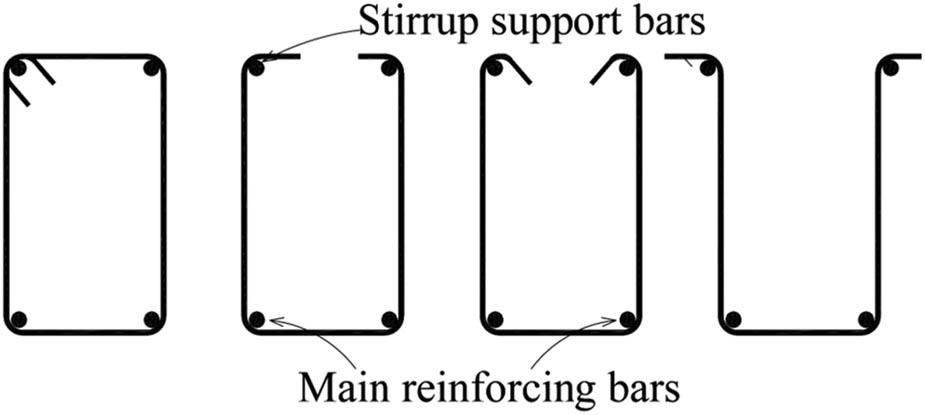
Bars in the compression area acting as stirrup hangers.
The rectangular cross-sections provided with both compression and tension steel reinforcement to resist bending moments are typically illustrated in code provisions and their manuals [3,12,13,14,15]. Many textbooks explain how to design these doubly reinforced concrete flexural members [9,16,17,18,19,20,21]. Also, several researchers deal with the analysis and design of such sections [8,22–26]. This analysis is, briefly, reviewed in the following sections.
Regarding a doubly reinforced beam, if the tensile reinforcement ratio (
As shown in Figure 1(e), the remaining tension steel
This can be rewritten using the definitions of
Hence, the total nominal moment is
To achieve the design strength, the nominal capacity is diminished by multiplying by the strength reduction factor ϕ = 0.90 if the net tensile strain
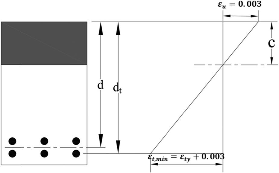
Minimum net tensile strain
For the reasons mentioned earlier, it is highly desirable that failure is caused by tensile yielding instead of crushing the concrete. Establishing a maximum threshold for the tensile reinforcement ratio can ensure this. Assuming the compressive steel reaches yield stress at failure, the tensile steel strain is established, which is equal to
The strength reduction factor ϕ is determined by the net tensile strain in the ACI Code [3] and not by the reinforcement ratio. If ϕ = 0.90, the maximum reinforcement ratio is
If
The aforementioned equations utilized for developing the basic analysis of doubly reinforced beams with simplicity and accuracy are applicable solely if the compression steel yields when the beam attains its nominal strength. In numerous instances, including shallow sections, wide sections, those utilizing high yield strength steel, sections with minimal tensile reinforcement ratio, or sections featuring thicker concrete cover over the compression steel bars, the compression stress in compression bars will remain below the yield stress at the failure state. Considering the scenario where the compression reinforcement has not yielded at the point of flexural failure in the doubly reinforced beam, more generally applicable equations must be developed. The following steps can be used to determine whether compression steel yields at failure. Considering
The minimum tensile reinforcement ratio (
If the tensile reinforcement ratio does not meet this limiting value, the neutral axis is elevated enough to prevent the stress in the compression steel at failure from surpassing the yield stress value. The balanced reinforcement ratio can easily be demonstrated using Figure 1(b) and (c) in this situation:
To calculate
Thus, the maximum reinforcement ratio allowed for ϕ = 0.9 is
By comparing equations (12) and (15), with
When the compression steel stress equals
The quadratic equation, with
The strength reduction factor ϕ is utilized to decrease this nominal capacity and achieve the design strength. The compression reinforcement becomes less likely to yield as the yield strength of the reinforcement increases. For example, the maximum strain in the concrete is 0.003, while the yield strain of Grade 100 reinforcement is 0.0034; therefore, Grade 100 reinforcement cannot yield in compression. To prevent compression bars from buckling outward under stress and causing spalling of the outer concrete, it is important to take precautions when using them in a flexural member. In ACI Code [3], reinforcement bars are required to be enclosed using closed stirrups or hoops, similar to the way compression bars in columns are enclosed by transverse ties. Transverse reinforcement is required along the entire length where compression reinforcement is necessary.
The first step is to check that the tensile steel ratio is lower than
To ensure beam yielding during failure, all doubly reinforced beams designed following the ACI Code [3] must be sub-reinforced by limiting the tensile reinforcement ratio. In Sections 2.1 and 2.2, two scenarios were discussed: (a) yielding occurs in both tensile steel and compression steel, and (b) yielding occurs in tensile steel while compression steel remains unyielded. Analyzing the capacity of the existing beams can result in two other combinations: (c) tension steel is not prone to yielding but compression steel is, and (d) neither type of steel is yielding. In reality, the last two cases are uncommon because creating such conditions would require a significant amount of tension reinforcement but the occurrence is possible. In these situations, the solution is obtained by simply extending the treatment of Section 2.2. An equation is created for horizontal equilibrium that uses the unknown neutral axis depth
Flowchart for the analysis of a doubly reinforced concrete section.
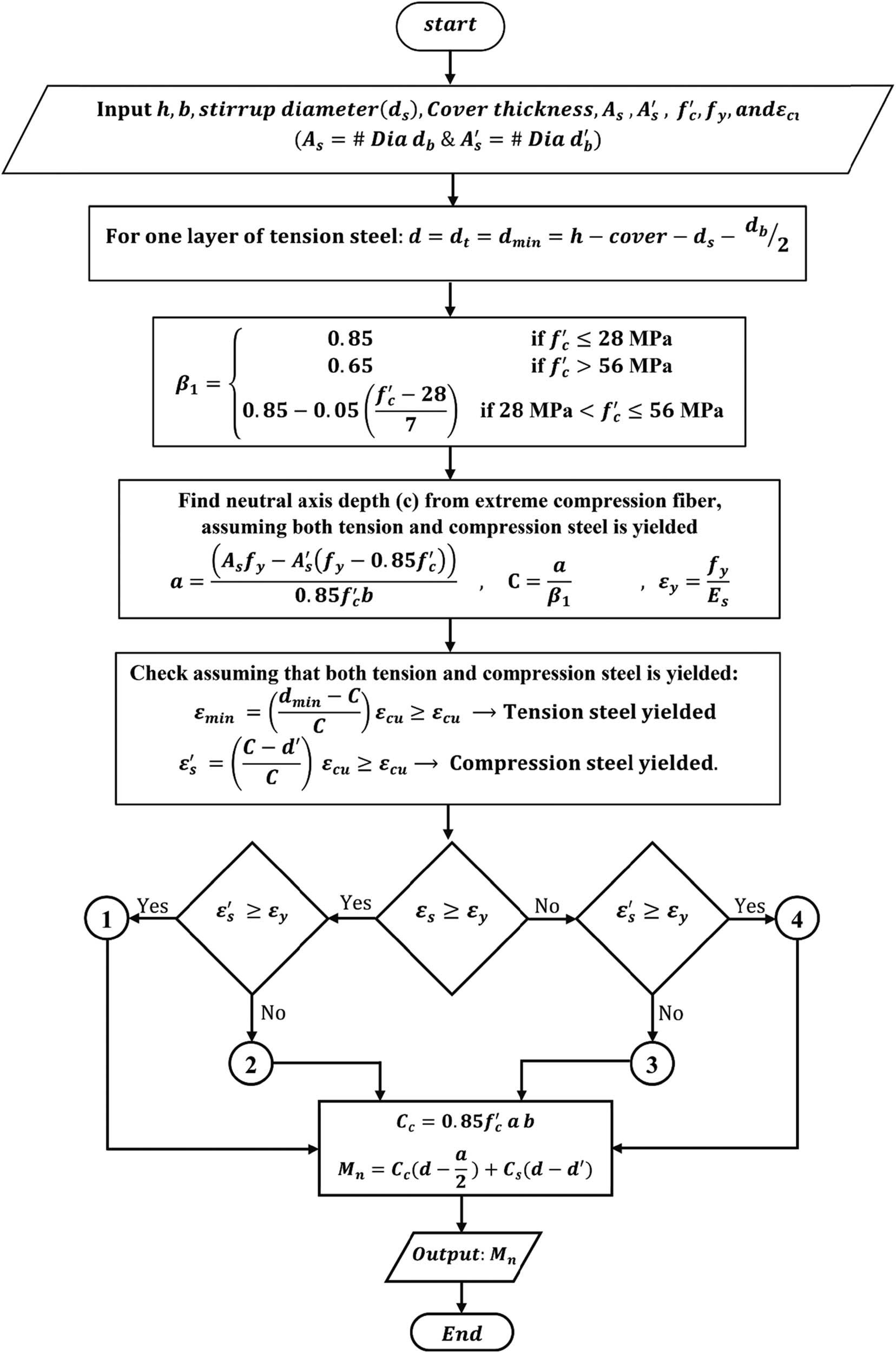
Figure 5 presents a comprehensive flowchart that outlines the systematic analytical procedure for evaluating doubly reinforced concrete sections. The flowchart begins with the fundamental assumption that both tension and compression steel have yielded, and then proceeds through a series of decision points to verify this assumption against the calculated strain values. The process involves checking whether the actual tensile reinforcement ratio exceeds the balanced reinforcement ratio, determining if compression steel reaches yield stress, and calculating the appropriate nominal moment capacity based on these conditions. This iterative approach ensures accurate prediction of section behavior by accounting for different failure modes – whether tension-controlled, compression-controlled, or balanced failure occurs. The flowchart serves as a practical tool for engineers to systematically analyze doubly reinforced sections while avoiding common analytical pitfalls that can arise when assumptions about steel yielding prove incorrect.
Figure 6 illustrates the detailed reinforcement configurations for the three experimental beam specimens (B1, B2, and B3) tested in this study. Each beam maintains identical overall dimensions of 1,750 mm span, 250 mm depth, and 100 mm width, with a consistent concrete cover of 8 mm and identical tension reinforcement consisting of two 22 mm-diameter bars. The key variable among the specimens is the compression reinforcement: B1 incorporates two 10 mm-diameter bars, B2 uses three 10 mm-diameter bars, and B3 employs two 22 mm-diameter bars, resulting in compression-to-tension steel ratios of 0.2, 0.3, and 1.0, respectively. The schematic clearly shows the positioning of both longitudinal reinforcement and transverse stirrups (10 mm diameter at 100 mm spacing), providing essential details for understanding the experimental setup. These configurations were specifically designed to investigate how varying amounts of compression reinforcement affect the structural behavior of shallow beams reinforced with high-strength Grade 500 steel, particularly their failure modes and ultimate load-carrying capacity.
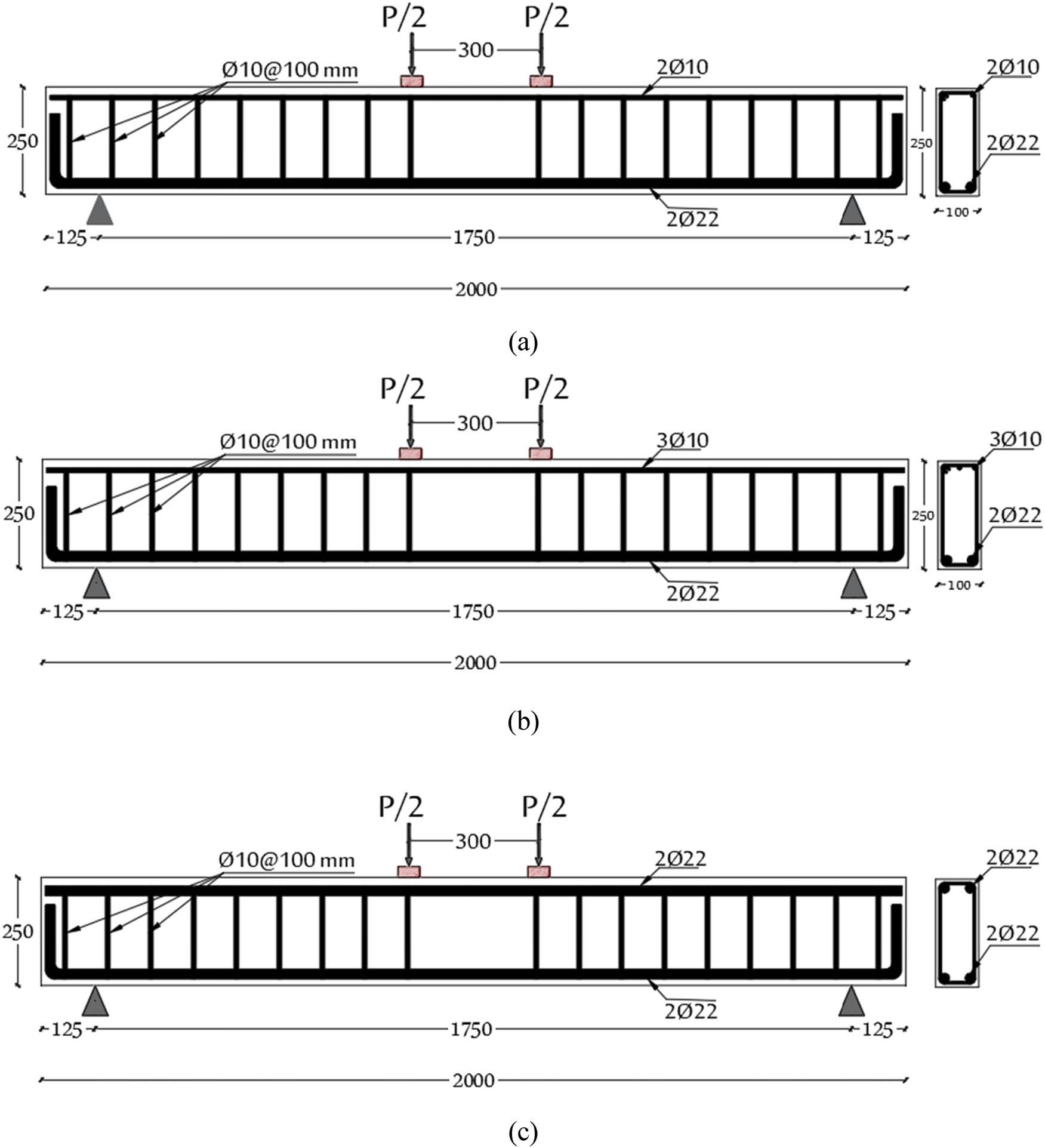
Schematic longitudinal and cross sections of the tested beams: (a) B1, (b) B2, and (c) B3 (all dimensions in mm).
Table 1 shows the concrete mix proportion for the specimen. According to ASTM C39 [27], the concrete mix’s compressive strength is 25 MPa. The cement used in the mixes was CEMI-52.5 N, in accordance with the European Standard EN [28]. This cement type was chosen for its high early strength development and consistent performance characteristics; type N (normal) designation provides a standard setting time suitable for laboratory casting procedures and complies with European Standard EN specifications, ensuring quality consistency. The fine aggregate utilized was natural siliceous sand, which meets the specifications outlined in EN196-1 [29]. The crushed dolomite stone was used as coarse aggregate in this investigation. This type was selected for its uniform mechanical properties and well-documented modulus of elasticity. Dolomite’s known aggregate modulus (typically 2–3 times that of cement paste) provides a predictable contribution to concrete’s elastic modulus calculations used in the proposed analytical method. A maximum size of 19 mm ensures adequate workability in the relatively narrow 100 mm beam width while maintaining representative aggregate-to-paste ratios. A high-range water-reducing Type F admixture was used. The water-to-cement ratio used in this study was 0.5. Three standard cylinders, each 300 mm in length and 150 mm in diameter, were manufactured and cured for 28 days under standard conditions until the test day. Deformed bars were utilized as reinforcement bars in this study, exhibiting a yield stress (
Concrete mix proportion (m3).
| Cement | Dolomite | Sand | Water | Admixture |
|---|---|---|---|---|
| 350 kg | 1,292 kg | 646 kg | 175 L | 5.4 kg |
The dimensions and reinforcing details of the RC beams are illustrated in Table 2 and Figure 6. Three RC beams were fabricated with a cross section of 250 mm in depth and 100 mm in width, with a total length of 2,000 mm. The thickness of the concrete cover was 8 mm. The tension reinforcement bars (two with a 22 mm diameter) employed in the beams were identical, as shown in Table 2. The compression reinforcement bars were changed in all the beams as the major parameters in this study, where B1 has two 10 mm-diameter, B2 has three 10 mm-diameter, and B3 has two 22 mm-diameter, as shown in Table 2. All the tested beams in this experimental study have the same constant parameters, including the loading, shear force, and bending moment diagrams, as shown in Figure 7.
Compression steel in the tested beams.
| Beam ID |
|
|
| Details |
|---|---|---|---|---|
| B1 | 2Ø22 | 2Ø10 | 0.2 | Figure 6(a) |
| B2 | 2Ø22 | 3Ø10 | 0.3 | Figure 6(b) |
| B3 | 2Ø22 | 2Ø22 | 1.0 | Figure 6(c) |
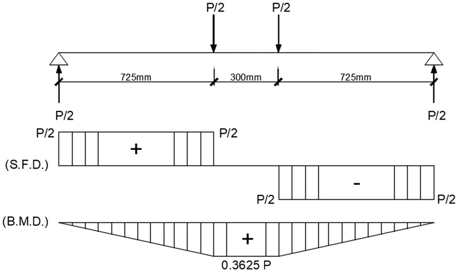
Loading, shear force, and bending moment diagrams of the tested beams.
The beams were cast following the guidelines outlined in ASTM C31 [31]. A portable vibrator was utilized to eliminate trapped air and achieve optimal compaction. Following casting, a trowel was employed to ensure that the surface of the beam was level. Subsequently, the beams’ surfaces were enveloped in moist burlap. The formwork was taken off after 24 h. The beams were cured for 28 days in accordance with ACI-308R-01-R08 [32]. Figure 8 shows the beam specimens and cylinders during concrete pouring. Reinforcement cages of the tested beams are shown in Figure 9.
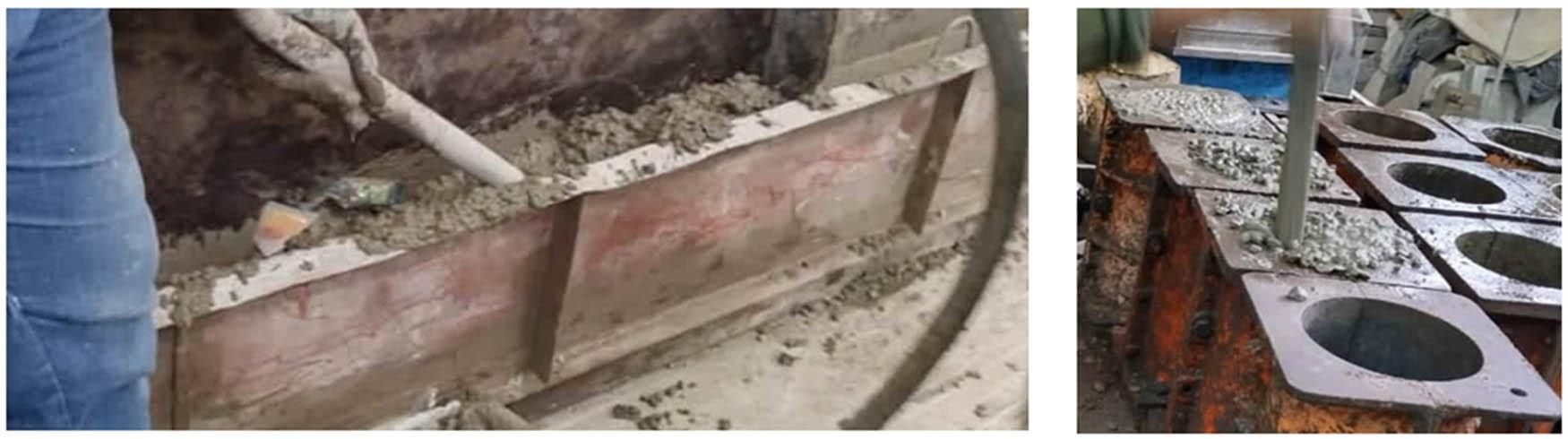
Concrete pouring of the beam specimens and cylinders.
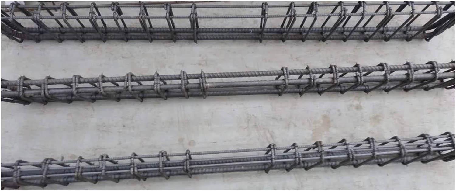
Reinforcement cages of beam specimens.
To assess the variance of strain as a function of the loading, five strain gauges were installed on every beam. One strain gauge, ST1 (Tokyo, gauge length 60 mm), was installed directly at the top of the concrete layer. Two strain gauges, designated as ST2 and ST3 (Kyowa, with a gauge length of 10 mm), were positioned at the upper reinforcement bar within the compression zone. Two strain gauges, ST4 and ST5 (Kyowa, gauge length 10 mm), were positioned at the bottom reinforcement bar. All gauge locations correspond to points of maximum expected strain in their respective materials. The measurement points align with the theoretical strain distribution assumptions used in the proposed analytical method. Placement enables direct comparison between experimental strain profiles and analytical predictions. For instance, ST1 is positioned at the extreme compression fiber to capture the maximum compressive strain in concrete. The longer gauge length (60 mm) averages strain over a representative concrete volume, reducing localized effects from aggregate distribution or surface irregularities. It is critical for validating the proposed analytical model’s assumption that failure occurs at εₒ ≈ 0.0015 rather than the conventional 0.003. In addition, ST2 and ST3 were positioned to directly measure whether compression reinforcement reaches yield strain (0.0025), which is fundamental to the analytical approach selection in the flowchart (Figure 5); ST2 and ST3 were strategically located in the maximum moment region where tensile strains are highest. The deflections at the midspan of the evaluated beams were measured using linear variable displacement transducers (LVDT). A data logger was employed to record the data from the LVDT and electrical strain gauges. Figure 10 shows the strain gauges used.
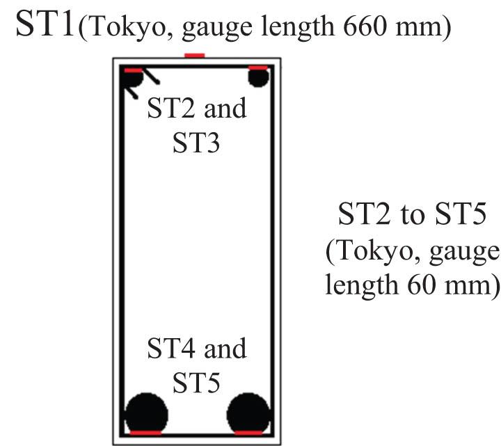
Positions of strain gauges.
The four-point flexural test was adopted for testing all beams with the central section subjected to pure bending, i.e., without shear effect. A Shimadzu Universal Testing Machine (UTM) with a 500 kN capacity was employed to load the beams monotonically. The crack propagation, mode of failure, and failure load for each beam were recorded. Figure 11 shows the test setup and locations of LVDTs. The clear span of the beam measures 1,750 mm, with the two loading points positioned 300 mm, symmetrically located around the midspan of the beam. The shear span measured was 725 mm for the tested beams. For each stage of loading, strains are measured at the maximum compression fiber of concrete, compression steel, and tension steel.
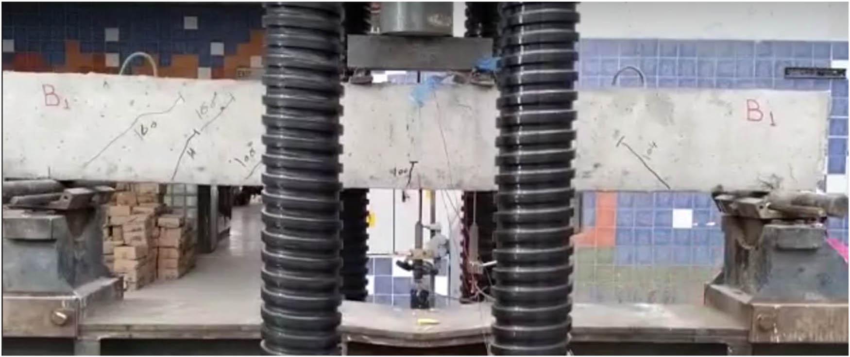
Test setup.
All beams experienced failure as a result of concrete crushing in the maximum moment region, as illustrated in Figure 12. In addition, all beams experienced compression-controlled failure, even B3, which has
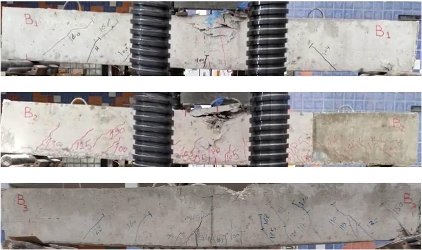
Compression-controlled failure of all the tested beams.
Figure 13 illustrates the load–deflection curves for all beams. The load–deflection response of all beams was approximately consistent. The load increase for the beams demonstrates nearly bilinear characteristics. Following the attainment of its maximum load, there is a notable abrupt interruption of the curves, as illustrated in Figure 13. This interruption can be attributed to concrete crushing in the compression region, resulting in its ultimate failure. Therefore, the test was terminated at this load level. Figure 13 illustrates that the B1 and B2 beams rapidly lose their capacity to support load shortly after attaining the peak load. Conversely, in the case of the B3 beam, there is a slight reduction in load immediately after reaching the peak load; however, the B3 beam continues to support the remaining load, as evidenced by the minor plateau that formed. Figure 13 and Table 3 demonstrate that the increase of steel bars in the compressive region significantly enhanced the load-carrying capacity of the beams. The B1 beam exhibited a failure at a peak load of 118.4 kN, whereas the B2 beam, which included 3Ø10, failed at a peak load of 122 kN, and the B3 beam had a peak load of 166 kN. The use of 3Ø10 in the B2 beam showed a slight increase in the load-carrying capacity by 3% compared to the B1 beam (with 2Ø10). In addition, the B3 beam (with 2Ø22) showed the highest load-carrying capacity compared to all beams, with an increased ratio of 40.2 and 36.1% compared to the B1 and B2 beams, respectively. The B3 beam demonstrated the capacity for further deflection beyond the peak load, a characteristic that was absent in the B1 and B2 beams. The B3 beam demonstrated a more significant deflection of approximately 3 mm following the attainment of the peak load and upon the onset of concrete crushing at the extreme top fiber. The test results are summarized in Table 3, including the load, maximum deflection, strain at maximum compressive fiber, strain at tension steel, and strain at compression steel at failure. The nominal moment strengths for all beams were calculated, as illustrated in Figure 7. The B1 beam had a nominal moment strength of 42.92 kN m, whereas 44.23 kN m for the B2 beam with 3Ø10, and 60.18 kN m for the B3 beam with 2Ø22. Using 3Ø10 in the B2 beam resulted in a 3% increase in the nominal moment strength compared to the B1 beam (2Ø10). The B3 beam (with 2Ø22) had the highest nominal moment strength among all beams, with higher ratios of 40.2 and 36.1% compared to the B1 and B2 beams, respectively.
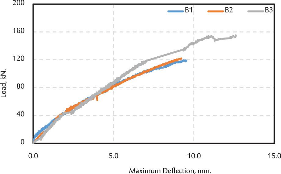
The relationship between load and maximum deflection for the tested beams.
Comparison of experimental and proposed method results.
| Point of comparison | B1 beam | B2 beam | B3 beam | ||||||
|---|---|---|---|---|---|---|---|---|---|
| Experimental | Analytical | % | Experimental | Analytical | % | Experimental | Analytical | % | |
| Failure load (kN) | 118.4 | 105.9 | +11.8% | 122.0 | 111.1 | +9.8% | 166.0 | 150.2 | +10.5% |
| Nominal moment strength* (kN m) | 42.92 | 38.39 | +11.8% | 44.23 | 40.27 | +9.8% | 60.18 | 54.45 | +10.5% |
| Concrete compressive strain at failure | 0.001526 | 0.001507 | +1.3% | 0.001413 | 0.001507 | −6.2% | 0.001518 | 0.001507 | +0.7% |
| Strain in tension steel at failure | 0.001376 | 0.001365 | +0.8% | 0.001460 | 0.001446 | +1.0% | 0.001765 | 0.001729 | +2.1% |
| Strain in compressive steel at failure | 0.001344 | 0.001330 | +1.1% | 0.001211 | 0.001194 | +1.4% | 0.000979 | 0.001054 | −7.1% |
*Bending moment due to the weight of the beam is neglected.
Figure 14 shows the relation between load and compressive strain in concrete till failure occurs. The curves increased almost linearly across all beams. No significant difference was observed between the B1 and B2 beams, while the B3 beam experienced a significant increase compared to the other beams. The most important result is that compression strain in concrete at failure is around 0.0015 and not 0.003 as in all provisions and codes. Figures 15 and 16 illustrate the load–strain curve for strain in tension reinforcement and strain in compressive steel, respectively, for the tested beams. The strains recorded by the strain gauges placed on both bars of the bottom and top (tension and compression bars) were approximately identical for each specified location, which was common for all strain gauges. The strain at every point was determined by averaging the values obtained from the two strain gauges associated with that specific point. For instance, the strain measured at the compressive reinforcement bars of the beam was calculated as the average of ST2 and ST3, while the average of ST4 and ST5 was for the tension reinforcement bars, as illustrated in Figure 10. The curves initially exhibit a linear progression, with B1 and B2 beams displaying identical trends with minor discrepancies. The B3 beam exhibits a significant disparity at the same deflection level. The curves for B1 and B2 beams exhibit a linear growth until they attain a load of roughly 110 kN. The load thereafter exhibits a minor increase before stabilizing, accompanied by a notable increase in strains. The B3 beam curve persists in a linear ascent until reaching a load of roughly 130 kN. The load thereafter exhibits a minor increase before stabilizing, accompanied by a substantial increase in strain. The curves indicate that the reinforcement bars in the tension zone have not yielded, as the strain values have not attained the yield strain threshold (0.0025), as illustrated in Figure 15. Regarding the strain in compressive steel, the same trends were noticed in tension steel, where the load–strain responses show a linear increase in the first part of the curves, and then the curves turn into a non-linear response, as illustrated in Figure 16. The curves demonstrate that the compressive reinforcement bars have not yielded, as the strain values have not reached the yield strain threshold (0.0025). Nonetheless, the results indicated that the strain values in the compression steel were lower than those in the tensile steel, as illustrated in Figures 15 and 16.
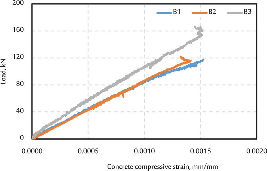
The relationship between load and maximum concrete compressive strain for the tested beams.
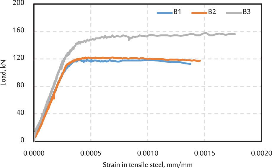
The relation between load and strain in tensile steel for the tested beams.
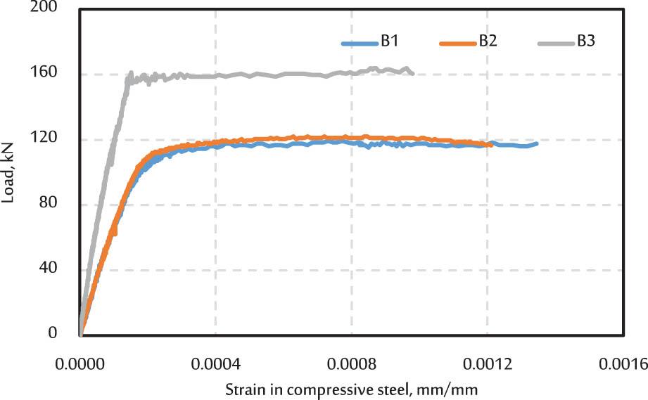
The relation between load and strain in compressive steel for the tested beams.
The load–deflection behavior observed in Figure 13 reveals fundamental differences in how these beams redistribute internal forces as they approach failure. The bilinear characteristics observed in all three beams reflect a two-stage loading process inherent to reinforced concrete behavior. (i) Initial linear stage: both concrete and steel behave elastically, with loads shared proportionally according to their respective elastic moduli. The slope of this portion corresponds to the composite section’s flexural rigidity (EI); (ii) second stage (reduced stiffness): as loads increase, concrete begins developing microcracks in the tension zone, progressively reducing the section’s effective moment of inertia. This creates the characteristic stiffness reduction visible in the curves. In addition, the plateau exhibited by B3 (
Analysis of the tested beams using the conventional method of such a doubly reinforced section, as shown in Figure 5, always fails. For example, starting with the assumption that both tension and compression steel yielded in the first trial does not match with the strains at the end of this trial, so in the second trial, we started with the strains at the end of the first trial, but, at the end, the strain in either tension steel or compression steel or both yielded. Therefore, we needed a third trial and so on, and the analysis did not converge, even after several trials. This could be due to many reasons, such as:
-
–
Strain at failure is almost equal to around 0.0015, not 0.003, as proposed by the code.
-
–
High-grade steel with a yielding stress = 500 MPa, accompanied by a shallow depth causes the impossibility of the compression steel to reach yielding.
-
–
Shallow depths also limit strain to reach the strain at which the section will be considered tension-controlled (0.003 + 0.0025 = 0.0055). The strain values for tension reinforcement bars may be less than the yield strain, so compression failure occurs in all three beams, even B3, which has
{{A}_{{\rm{s}}}=A}_{{\rm{s}}}^{^{\prime} }
Therefore, the conventional calculations could not be used in these shallow beams reinforced by high-grade steel with a yield stress equal to 500 MPa. Building codes, including those from the ACI code [3], generally specify a 0.003 as the maximum compressive strain of concrete subjected to flexural load. This value represents a simplified and conservative estimate that considers the intricate stress–strain behavior of concrete to ensure a margin of safety. Although 0.003 is commonly applied in designs, the actual strains at failure were different. The actual strain at concrete failure is influenced by factors such as the concrete mix, reinforcement grade, and reinforcement confinement. Consequently, it is imperative to develop an analytical approach that ensures high precision, particularly for the design of doubly reinforced shallow beams utilizing grade 500 steel.
From the above discussion of the results, it is obvious that the conventional calculations of such shallow beams are not suitable for determining their flexural capacity, especially if they are reinforced by high-grade steel. In this research, the authors developed a proposal to analyze these sections.
First, we determined the value of the modulus of elasticity of concrete,
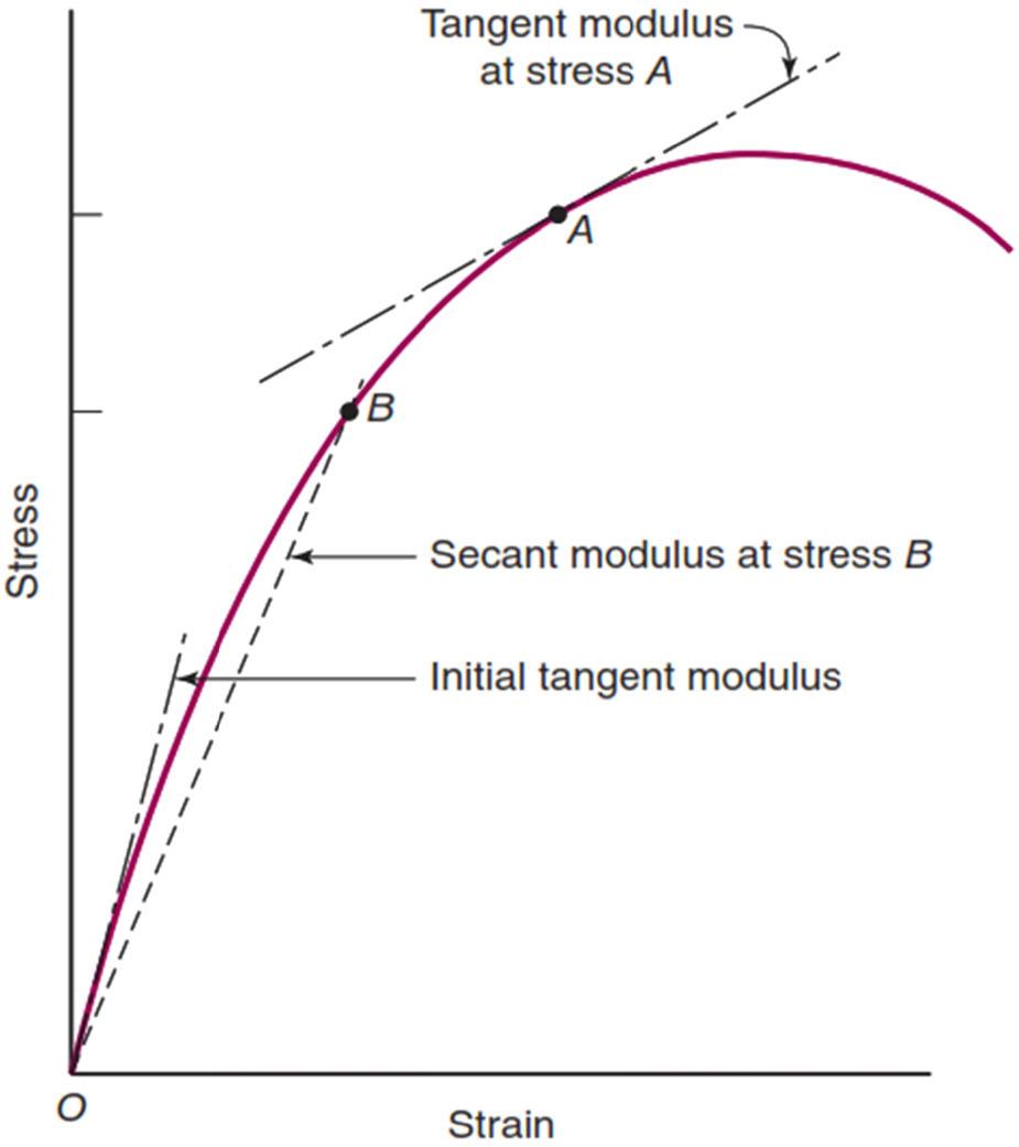
Initial, tangent, and secant moduli of elasticity of concrete [9].
The initial tangent modulus of elasticity, the initial slope of stress–strain curves, increases with increased compressive strength. The modulus of elasticity of concrete (
This formula, derived from short-term tests on concrete within the specified density range, represents the secant modulus at approximately 0.50
For normal-weight concrete, the ACI Code provides [3]
Additionally, ACI Committee 363 [34] suggests the following for high-strength concretes:
Equations (19)–(21) offer practical means to estimate concrete’s modulus of elasticity based on its compressive strength and density.
Figure 18 presents standard stress–strain responses for concretes with varying strength classifications, derived from approximately 15-min tests on specimens analogous to a beam’s compression zone. These curves exhibit an ascending branch that peaks at maximum stress, corresponding to strains ranging from 0.0015 to 0.003, subsequently followed by a descending segment. The shape of the ascending branch is attributed to the gradual development of microcracks within the concrete’s structure. Notably, five key properties can be identified from these curves, which are instrumental in formulating mathematical models for concrete’s compressive stress–strain behavior [35].
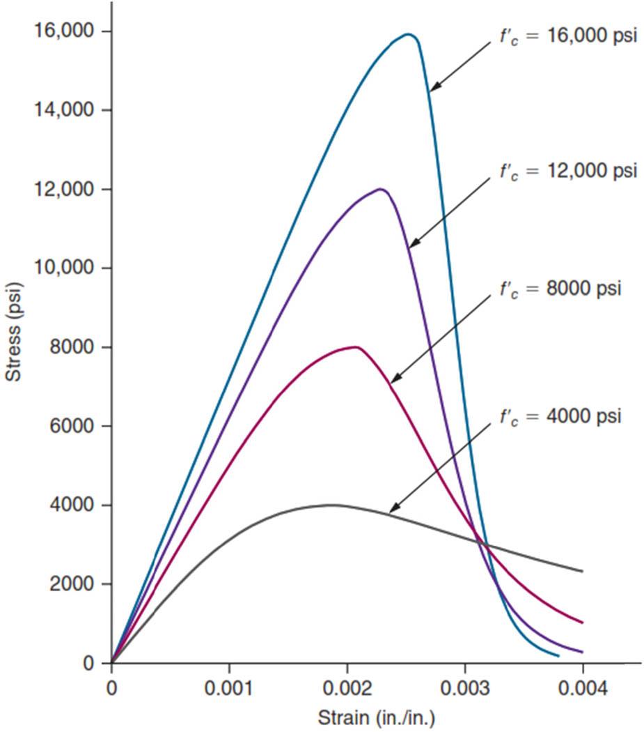
Typical concrete stress–strain curves in compression [9].
The ascending segment of the concrete stress–strain curve is often approximated by a parabola peaking at the maximum stress [35,36]. This parabolic approximation is commonly employed for computational purposes. As concrete strength increases, the ascending portion of the curve tends to straighten [37]. As concrete compressive strength increases, the strain at maximum stress (
The modified Hognestad stress–strain curve [9] is a widely accepted model for representing the behavior of concrete under compression, particularly for concretes with strengths up to approximately 42 MPa. This model provides a parabolic approximation of the ascending portion of the stress–strain curve, as depicted in Figure 19, culminating at the peak stress, and is commonly used for computational analyses.
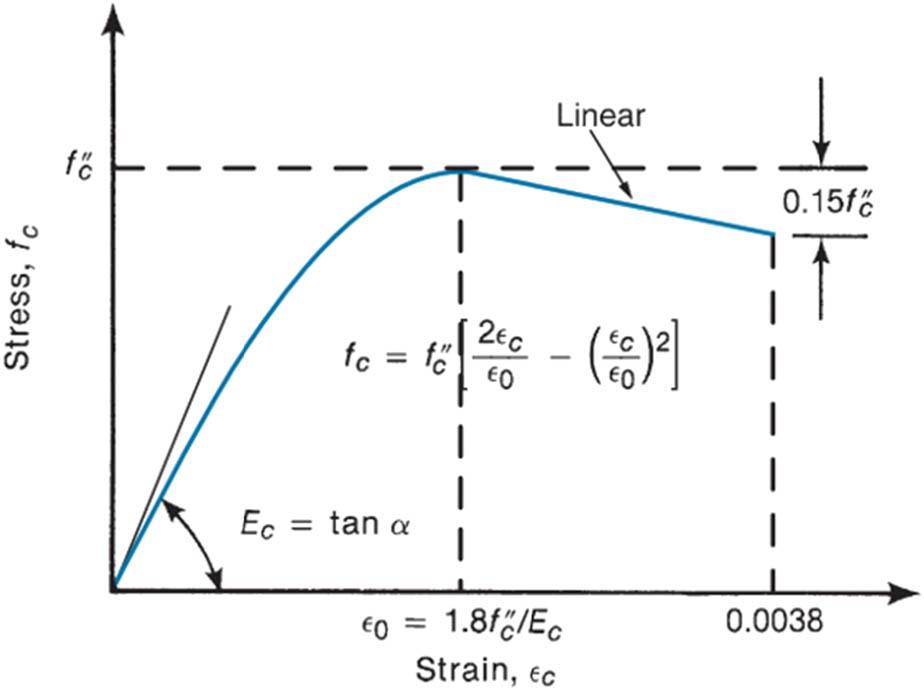
Analytical approximation to the compressive stress–strain curve for concrete [9].
The experimental results indicate that shallow beams fail once the concrete compressive strain reaches
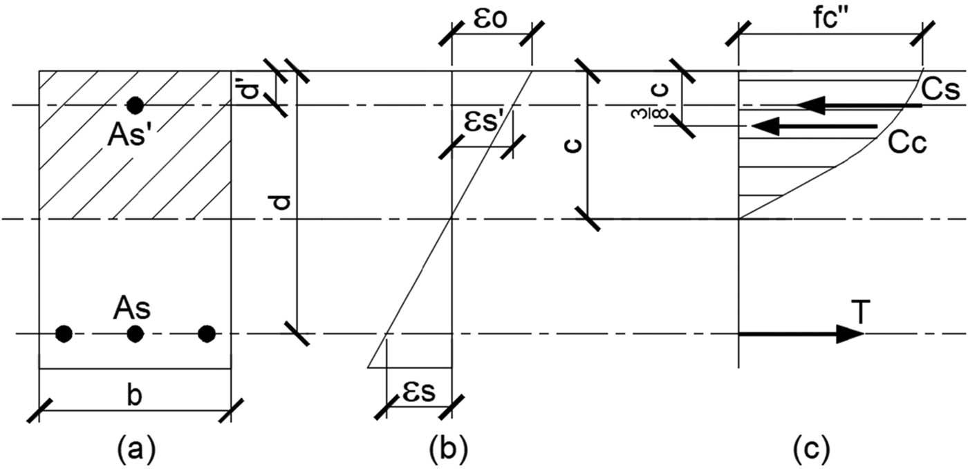
Proposed analytical model for shallow beams. (a) Cross-section, (b) Strain distribution, and (c) Stress and forces.
In this analysis,
As shown in Figure 19,
In this investigation,
In the proposed analysis method, the equations are consistent with those presented in Figure 5, with the following key differences:
-
Compressive force in concrete (
{C}_{{\rm{c}}} (24) {C}_{{\rm{c}}}=\frac{2}{3}\times 0.9{f}_{{\rm{c}}}^{^{\prime} }\times c\times b=0.6{f}_{{\rm{c}}}^{^{\prime} }\times c\times b. -
The location where the concrete compressive force is applied is as follows: Unlike conventional beams, where the compressive force is assumed to act at the centroid of a rectangular stress block (typically at
a/2 3/8c -
Compressive force in steel reinforcement (
{C}_{{\rm{s}}} {f}_{{\rm{c}}}^{^{\prime} } {f}_{{\rm{c}}}^{^{\prime} }
In equation (25), if the compression steel reaches its yield strain, the yield strength (
These adjustments aim to provide a more accurate representation of the actual stress distribution within the concrete and the contribution of the steel reinforcement.
The primary outcomes of the proposed analytical method, alongside the corresponding experimental findings, are summarized in Table 3. The analysis of the experimental results compared to the analytical results proposed by the authors indicates the following:
-
The strains are very similar, exhibiting an error of approximately 7%.
-
The difference in the ultimate load or the maximum bending moment the beam can withstand is within approximately 11%, with the experimental results being higher than the analytical calculations.
The error percentages were calculated using the standard relative error formula:
They show remarkable consistency (8.9–10.6% range), indicating the proposed method’s reliability across different compression steel ratios. The results are generally consistent, except for B3 compression steel strain (7.7% error). This outlier is likely to reflect the higher sensitivity in compression steel behavior at
Accordingly, the proposed calculations can predict the strength of these shallow beams reinforced with high-strength steel, yielding results on the safe side compared to traditional calculations, which fail to provide an accurate analysis for such beams.
Sometimes, architectural considerations require the use of hidden beams instead of projected beams. As a result, the beam depth is limited by the depth of the concrete slab, making it necessary to use compression reinforcement, which may be equal to the tensile reinforcement, to compensate for the reduced concrete section depth. If these shallow beams are reinforced with high-yield-strength steel (500 MPa), traditional calculations are not suitable for predicting the beam section’s resistance to bending moments. This is because the beam fails before the maximum strain in the concrete on the compression side reaches 0.003, as specified in most design codes. Experimental tests were conducted on three beams to investigate their behavior, with the compression reinforcement ratio to tensile reinforcement set at 0.2, 0.3, and 1.0. The strains in the concrete, tensile reinforcement, and compression reinforcement were measured, along with the failure load of these beams. Instead of the conventional method, a proposed method has been developed to analyze these sections. The proposed analytical calculations accurately predict the strength of shallow beams reinforced with high-strength steel, as evidenced by the close agreement between experimental and analytical strain results and the slight (approximately 11%) conservatism in ultimate load predictions, ensuring a safer assessment compared to traditional methods. From the above, it is evident that using high-strength steel on the compression side along with steel on the tension side in shallow beams, even if their ratio is 1, will not solve the issue of compression-controlled failure. Such failure will still occur, making this solution uneconomical. This is because the strain in both the tension and compression reinforcement will likely not reach the yield strain, meaning we will not fully utilize the strength of the used steel. Additionally, a reduction factor of ϕ = 0.65 will be applied instead of ϕ = 0.90, which is used in tension-controlled failure. This means that we will only utilize 72% of the strength that could have been used, making this solution highly uneconomical. Therefore, it is not recommended unless absolutely necessary.
The authors recommended expanding this study through the following:
-
Phase 1: Investigating the parametric studies, such as the effects of beam depth, steel grade, and reinforcement ratio, to develop specific correction factors and analytical models.
-
Phase 2: Studying the influence of material properties, such as concrete strength and aggregate type, on reinforcement efficiency.
-
Phase 3: Focusing on design optimization through cost analysis and the exploration of alternative solutions like high-strength concrete.
-
Phase 4: Developing simplified design guidelines and support code modifications for the practical application of the findings.
The authors gratefully acknowledge the funding of the Deanship of Graduate Studies and Scientific Research, Jazan University, Saudi Arabia, through Project number JU-202503163-DGSSR-RP-2025.
All authors contributed to the work equally.
Authors state no conflict of interest.
The datasets generated during the current study are available from the corresponding author on reasonable request.