
In this study, we aimed to determine the suitability of several of the most used interpolation methods for constructing isopleth maps. This is important because isopleth maps are designed to visualize the spatial distribution of the values of many different statistical indicators, which have different characteristics. Therefore, highly rated interpolators for visualizing physical phenomena are often not equally effective for statistical indicators.
The numerical value range of an indicator is an important feature, which should fall within a certain range. Examples include population density, whose value cannot be less than 0, and forest cover between 0 and 100%. Exceeding these limits makes the mapping model of the phenomenon inaccurate.
The numerical value range is also important because of the need to maintain the category volume on the map. This is the same as maintaining statistical consistency with the database. Therefore, it is important to check which interpolation method results in the smallest errors.
The third factor affecting the readability of isopleth maps is their appearance. The shape of the isopleths, their co-shape, and the smoothing of the course all affect this and the ergonomics of their use. Evaluating the usefulness of the method can be performed by surveying readers of isopleth maps. Map user preferences can then be considered as a complementary criterion for selecting an interpolation method. Conclusions from such a broad-based evaluation can increase map reliability with a strategic interpolator choice. In this context, the utility of the interpolation method is greater.
Improving isopleth maps began as early as the second half of the nineteenth century shortly after Ravn’s first application of the method. Two approaches were taken: the first, known as geographic interpolation, consisted of modifying the course of the isolines according to the map maker’s expertise (Mościbroda 1975). The second approach focused on the mathematical properties of interpolation – an example being the so-called interpolation scales by F. Uhorczak. They reflected different perceptions of the nature of isopleth maps. The first was built on an approach that relied on topographical map reading. The second approach recognized their ability to show key trends and gradients. Understanding isopleths as a mathematical construct is a concept first recognized by Greim (1912). However, it was not until the second half of the twentieth century that this view became dominant (Board 1967; Cebrykow 2004; Mościbroda 1999; Robinson 1961). Therefore, the criteria for the correctness of these maps were redefined accordingly. Preserving the volume of the phenomenon on a map as a solid form using a statistical surface has received considerable attention (Cebrykow 2004; Kyriakidis 2004; Lam 1983; Lin et al. 2016; Mościbroda 1999; Tobler 1979). However, applying these conditions is limited to indicators with spatial continuity.
Three different research approaches were used to improve the volume of these phenomena. These involved determining the optimal base field, its point representation and how to interpolate the statistical surface (Bracken & Martin 1989). The properties of the basic field are a broader problem and touch on other modes of cartographic representation (Do et al. 2015). To date, research has predominantly focused on the shape of fields and their layout and area in conjunction with their representation (Barnes 1978; Colette et al. 2010; Craig & Adams 1991). Conclusions can be drawn based on some recent studies indicating that regular hexagons are an optimal choice (Karsznia et al. 2021; Luo et al. 2019; Puu 2005).
Searching for improved solutions in the field of interpolation is most often performed in the context of physical phenomena (Comber & Zeng 2019). Therefore, those developed with isopleths in mind have been cited first. Initial research in this field was conducted in Poland by Prof. Uhorczak (Sirko & Mościbroda 2002). The precursor of volume-preserving interpolation was examined by W. Tobler (Tobler 1979), the author of the pycnophylactic method. However, this interpolation approach is still being developed (Cebrykow 2005; Gastner et al. 2022; Kim & Yao 2010; Mohammed et al. 2012; Rase 2001; Yoo et al. 2010) and the proposed solutions have not yet become standard. To date, there has been extensive comparative research into the more popular interpolation methods (Comber & Zeng 2019; Li & Heap 2014; Raghuvanshi & Tiwari 2023; Tan & Xu 2014). In some studies, kriging has received higher ratings (Liu & Yan 2021; Raghuvanshi & Tiwari 2023; Zimmerman et al. 1999). Meanwhile, in other applications, kriging, IDW and local polynominal have been rated equally high (Antal et al. 2021). There are also examples of IDW (Karp et al. 2024; Meng & Borders 2013; Perello & Simoes 2017) or linear interpolation being identified as the most effective solutions (Workneh et al. 2024).
In summary, it is difficult to select one single universal interpolation method, with the most used being kriging, IDW and linear interpolation. Each method has advantages and disadvantages, which become more apparent with changes in spatial organization and sampling density of the data (Li & Heap 2014).
Isopleth maps created using data downloaded from the Central Statistical Office (GUS) formed the basis of the current research. Two indicators were selected to describe population density and forest cover related to the administrative divisions at the municipality level. The population and forest cover data were from 2023. The data was integrated with the 2023 administrative divisions of Poland obtained from GEOPORTAL.
The study method comprised the following steps:
- –
preparing the database
- –
constructing test maps
- –
measuring the volume of the phenomenon and consistency of data values
- –
survey evaluation of the maps.
Preparing the database consisted of assigning values to municipalities. Then, points representing the communes were generated, located in the centre of gravity. The principle of a single-point representation of the area was used. The field value was attached to each point as an indicator. The data were transformed in QGIS.
The next stage consisted of developing isopleth maps for testing. For this purpose, the Surfer 24 programme (Golden Software) was used with six interpolation methods. It was assumed that in the execution of all maps, the changeable parameters would have default values.
The consistency of the range of values obtained using interpolation was determined and compared with the original data range. The next test only included maps of population density values for which the volume of the phenomenon was calculated. In the case of the population density index, the volume could be interpreted as the population number attributed. The calculated values were then compared with the total population of Poland.
The third element of the study was a survey to establish which map was the most user-friendly. The surveys were conducted among geographers in person, except for one survey that was conducted by phone. This group was selected based on the need to obtain findings based on the opinions of professionals familiar with map reading. The survey referenced two charts showing the distribution of population density and forest cover values in Poland, on which six maps developed using the interpolation algorithms being examined were placed (Fig. 1, 2). Twenty-five respondents participated in the survey, which, under the assumptions presented, ensured sufficient reliability of the results (Medyńska-Gulij 2024). The participants answered the following five questions:
Rate each map on to what extent it reflects the correct distribution of the phenomenon
Rate how quickly you can read the distribution of the phenomenon’s values on the map
How would you rate the level of consistency and graphical order
Rate the level of acceptance for the statement: the map effectively represents the spatial distribution of the indicator values
Specify how the level of generalization on the map was selected.
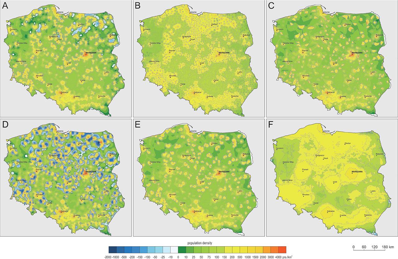
Test chart containing six population density maps made using six interpolation methods: (A) kriging, (B) IDW, (C) linear interpolation, (D) minimum curvature, (E) natural neighbour and (F) local polynominal
Source: own study
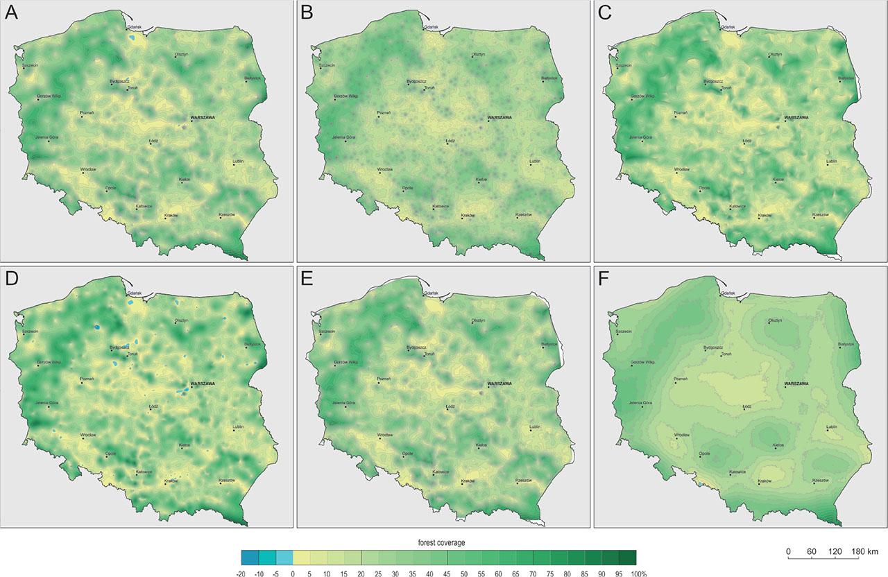
Test chart containing six forest cover maps made using six interpolation methods: (A) kriging, (B) IDW, (C) linear interpolation, (D) minimum curvature, (E) natural neighbour and (F) local polynominal
Source: own study
Responses were scaled using the five-degree Likert scale (Darnton 2023), which is often used in survey research and cartography (Wielebski & Medyńska-Gulij 2023).
It was verified that the statistical plots obtained represent values identical to the original data. In addition, it was confirmed that they were not outside the range of mathematical correctness for the given indicator. In the case of forest cover, the values must lie within a closed interval between 0 and 100%. The input data describing forest cover in Poland referred to municipalities and ranged from 0% to 88.3%. In the case of the population density indicator, the achievable values needed to be greater than zero, and the values of the original data oscillated between 4.2 and 4099.5 prs./km2.
In the study dataset, three interpolation methods, that is, IDW, linear interpolation and natural neighbour allowed the correct reproduction of the extreme values of the forest cover index and the population density (Tab. 1). The other methods, namely, kriging, minimum curvature, and local polynomial, resulted in changes in the range of indicator values.
Range of values of statistical plots representing forest cover and population density for six interpolation methods
| Data range | Interpolation method | |||||
|---|---|---|---|---|---|---|
| kriging | IDW | Linear interpolation | Minimum curvature | Natural neighbour | Local polynominal | |
| forest cover [%] | −0,6–90.7 | 0.01–88.3 | 0.05–88,3 | −20.9–103,8 | 0,05–88,3 | −3,36–91,4 |
| population density [prs./km2] | −140,9–4049,7 | 4,3–4067,4 | 4.3–4055,9 | −1847.9–4331.2 | 4.3–4026.1 | −148,5–836,3 |
Source: own study
Underestimation of the lower limits for two indicators for kriging, minimum curvature and local polynomial exceeded the zero value and was strongest for the minimum curvature method. The change in the upper limit was an increase in the forest cover value and a decrease in the population density value. The largest change in the data value range was brought about using the local polynomial method. The range of differences in the spread of the values of the statistical areas is presented in Fig. 3.
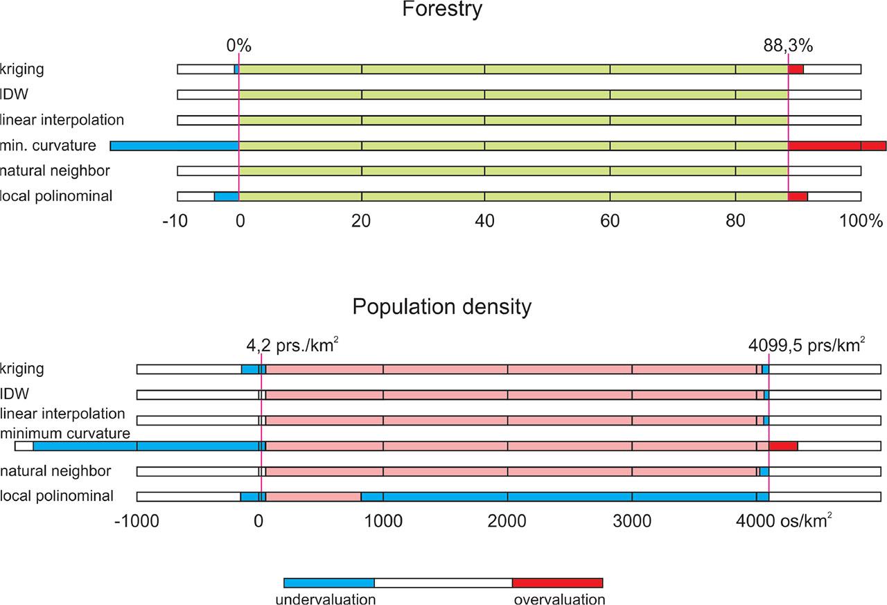
Differences in the range of values in maps of population density and forest cover for six interpolation methods compared to source data
Source: own study
The next study concerned calculating the volume of the phenomenon (Tab. 2), which could only be performed for the population density index. The volume of this cluster could be equated to the population of the area being examined. The results indicate that there was an overestimation of this figure in the range of 24.7% to 111.7%. This corresponds to a population ranging from approximately nine to over 42 million. The smallest error was recorded for the minimum curvature method, with a slightly greater level of error for linear interpolation and natural neighbour. The volume was overestimated the most when kriging was applied.
Statistical volume of maps depending on the interpolation method used compared to the population of Poland
| Interpolation method | ||||||
|---|---|---|---|---|---|---|
| kriging | IDW | Linear interpolation | Minimum curvature | Natural neighbour | Local polynominal | |
| Volume [= residents] | 79 950 779 | 58 054 424 | 48 799 862 | 47 098 511 | 48 865 153 | 60 842 675 |
| too much about | +42 184 449 | +20 288 094 | +11 033 532 | +9 332 181 | +11 098 823 | +23 076 345 |
| Error [%] | 111, 7 | 53,7 | 29,2 | 24,7 | 29,4 | 61,1 |
Source: own study
The analysis of the usefulness of the selected interpolation methods was supplemented by a questionnaire (Fig. 4). The best results in rendering the spatial distribution of indicator values (Question 1) were achieved using the natural neighbour method (pop. density 84% and forestry 80%). This was followed by linear interpolation (56% and 48%) and IDW (52% and 56%). The map made using kriging was only accepted for showing the forest cover (68%). In contrast, using the local polynominal method received a negative reception at 72% and 48%. The results obtained were largely confirmed in the answers to Question 4, which was included as a control question.
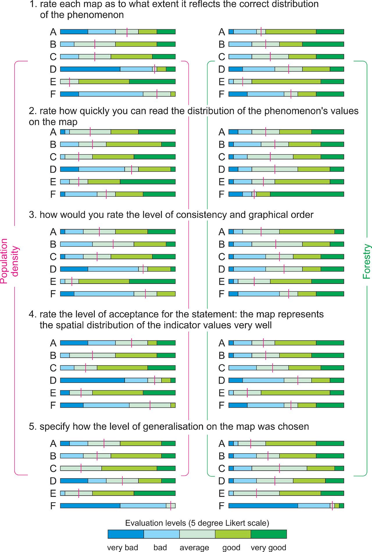
Graphical visualization of the survey results. Letters indicate interpolation methods: A – kriging, B – IDW, C – linear interpolation, D – minimum curvature, E – natural neighbour, D – local polynominal. The red line indicates the neutral position
Source: own study
The speed of reading the map was explored in Question 2. The maps were rated at a similar level in the case of forest cover except for the minimum curvature method, which was read by far the fastest (76%). Greater differences were found for the population density maps. The natural neighbour method was rated the best at 76% and 60% and the map produced using the local polynominal method was the slowest to read.
Consistency of construction and graphical order was also assessed. The best results were obtained using the natural neighbour method at 72% for both indicators, followed by kriging at 52% and 56%, linear interpolation at 56% and 44% and IDW at 36% and 36%. The maps made using the minimum curvature method with 68% and 32% negative indications and local polynomial with 64% and 44% negative indications received the lowest ratings.
The last point concerned the evaluation of the level of generalization. Here, for population density, the natural neighbour method was rated the best (72%), followed by linear interpolation (64%) and IDW (56%). For the forest cover maps, kriging (68%), IDW and natural neighbour (56% each) performed best. The local polynominal method received the lowest acceptance with 92% and 88% of responses being negative.
Considering the consistency of the values of the interpolated statistical plots, the results are similar for the forest cover and population density index. The correctness of the representation of the forest cover index values by the three interpolation methods can be recognized, that is, IDW, linear interpolation and natural neighbour. Small deviations from the original range of values could be considered insignificant. Similar conclusions could be drawn for the range of population density values. However, the trend towards an increase in the minimum value and a decrease in the maximum value should be noted. However, these changes are not of large magnitude, would not be visible on a map and can only be ascertained using a mathematical statistical surface model. With the lack of full correspondence of the data range in the surface obtained using linear interpolation, this should be the case but may raise doubts. This can be explained by creating a data model in Surfer, which involves creating a grid whose nodes do not faithfully reproduce the position of the feature points.
The criterion of consistency for the spread of data values indicates that the use of the other interpolation methods, that is, kriging, minimum curvature and local polynominal, may result in errors. These are particularly unacceptable when the values fall outside the maximum range of values. The largest errors were recorded for the minimum curvature and local polynominal methods. Kriging introduced small deviations extending the range of values. Additional conditions introduced in the algorithm settings would result in better results that keep the indicator values within an acceptable range (Yoo et al. 2010). These changes in the range of data values are because of the nature of algorithms that use the principle of spatial trending. For example, kriging was developed to detect the highest concentration of ore in deposits. However, the advantage of such applications does not work when analyzing the distribution of field-referenced statistical values. The location of points representing the basic area is another reason for the under- or overestimation. The points representing urban and rural areas are often located relatively close to each other. There are high gradients that are particularly evident in the population density indicator, which contributes to the formation of deep statistical depressions.
Evaluating algorithms for modelling statistical surfaces through the prism of preserving the volume of a phenomenon seems strategic and easy to verify. However, this only makes sense with statistical surfaces describing continuous phenomena. The concordance of the volume allows the statistical validity of the map to be ascertained but does not allow it to be assessed in terms of the level of generalization. Therefore, the overall volume is one of the prerequisites for mapping accuracy. In this context, additional criteria should be introduced when evaluating the maps and interpolation algorithms.
All the interpolators overestimated the volume of the phenomenon in the current study. The lowest error values were obtained for minimum curvature, and slightly higher errors were obtained for linear interpolation and natural neighbour. The largest overestimation, reaching almost 112%, was obtained with kriging. This result may seem surprising, especially as in many publications this method is well appreciated and is the most widely used (Rakotonirina et al. 2024). However, it should be emphasized that, to date, the research on the algorithm has mainly focused on evaluating maps of physical phenomena. Statistical indicators are different and the distribution of values is difficult to verify, in contrast to the physical phenomena. However, in the literature, arguments can be found for almost identical interpolation results when kriging and pycnophylactic, when the parametric settings of the algorithm are modified (Yoo et al. 2010).
In the study on usability, additional criteria were used based on users’ subjective evaluation of the maps. This is particularly relevant when maps are only used in the form of a graphic model. The results positively identified the use of natural neighbour, followed by linear interpolation and IDW. Kriging only gained recognition for data with a smaller spread of indicator values. Evaluations of the graphical consistency of the map construction, as expressed by the smoothed surface and the co-shaping of the isolines, yielded similar results. This confirms the opinion that the attractiveness of the graphic form of a map positively influences its reading (Medyńska-Gulij 2024). This is why the methods of IDW and linear interpolation were assessed as being less effective because IDW is burdened with the frequently occurring ‘bull’s eye’ effect (Li et al. 2017) and linear interpolation is characterized by isolines with a broken course.
The usability study overlooked computational efficiency in the evaluated algorithms, despite its potential importance when selecting an interpolation method. In this study, execution times varied from 0.04 s for linear interpolation to 29.4 s for kriging, with most methods completed within 10 s. The dataset comprised 2,556 records, generating a grid of over two million points. All the computations were performed on a standard PC with 16 GB of RAM and a quad-core processor. Consequently, computational time was not a limiting factor in this study. However, for larger datasets, efficiency considerations are likely to become increasingly important.
The study was conducted using data on population density and forest cover in Poland. However, the criteria used to evaluate the properties of statistical areas have an objective value and can be applied to other regions worldwide. Extending the conclusions to density-based indicators is justified, whereas percentage-based indicators present a more complex issue. It can certainly be assumed that the conclusions apply to all percentage indicators representing the proportion of a given area, such as forests, grasslands and orchards. However, in the case of demographic or economic indicators, negative values may occur, which limits the applicability of the obtained results.
Taking all three evaluation criteria into account, the best interpolation method cannot be unambiguously identified. However, considering the survey results, several conclusions were reached:
There is no universal interpolation method for all applications.
For interpolation of percentage and density ratios, the best results were achieved using linear interpolation followed by natural neighbour and IDW.
Kriging has great potential in isopleth mapping using variable settings inside the interpolation procedure. This requires further research.
The indications obtained may contribute to wider use of isopleth maps, especially since they have been well evaluated alongside other cartographic presentation methods (Słomska-Przech & Gołębiowska 2021).