
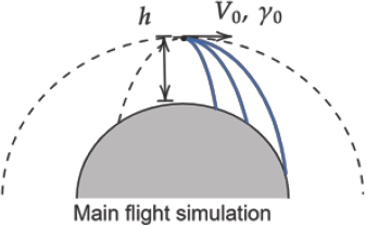
Fig. 1:
Initial conditions for the re-entry simulation.
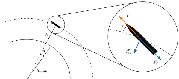
Fig. 2:
Diagram of the re-entering projectile.
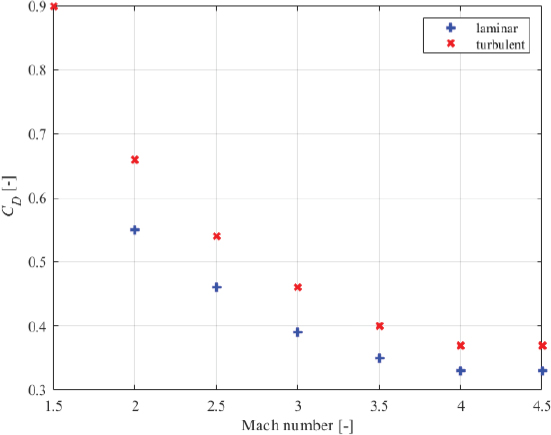
Fig. 3:
Drag coefficient (CD) vs. Mach number for the XM110 projectile for both laminar and turbulent flow. This graph is based on data collected by Braun (1973).
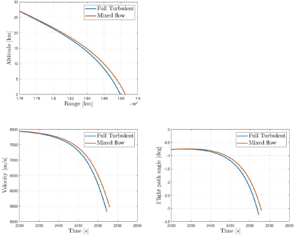
Fig. 4:
Flight trajectory (a), velocity (b) and path angle (c) to test the influence of the Reynolds number.
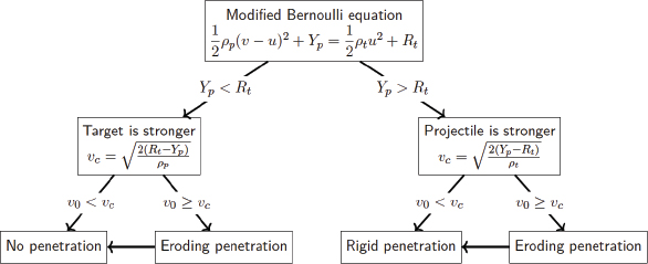
Fig. 5:
Penetration mechanisms.
Tab. 1:
Overview of relevant material properties.
| Material | ρt [kg/m3] | Rt [GPa] | |
|---|---|---|---|
| 7 ksi Concrete [HJC] | 2,440 | 48 | - |
| SAC5 Concrete [N et al.] | 2,299 | 37.9 | - |
| WSMR-5 3/4 Concrete [SYG] | 2,299 | 44.8 | - |
| 3.7 ksi Concrete [SYG] | 1,990 | 25.5 | - |
| Concrete [VLK] | 2,300 | 51 | - |
| Limestone [VLK] [WHP] | 2,300–2,320 | 58–63 | - |
| Sandstone [B et al.] | 2,000–2,040 | 16–30 | - |
| Steel [T] | 7,850 | - | 3.45–5.18 |
1 Data sources are – for concrete: Butler, Nielsen, Dropek & Butters (1977); Holmquist, Johnson & Cook (1993); Warren, Hanchak & Poormon (2004); Noble, Kokko, Darnell, Dunn, Hagler & Leininger (2005); Stokes, Yarrington & Glenn (2005); Vahedi, Latifi & Khosravi (2008); and for steel: Tate (1986).
This table is inspired by the work of Flis (2016).
Tab. 2:
Overview of material properties with dynamic penetration parameters.
| Material | Rt [MPa] | Yp [MPa] | ||
|---|---|---|---|---|
| Concrete (lower boundary) [SYG] | 1,990 | 25.5 | 362 | - |
| Concrete (upper boundary) [VLK] | 2,300 | 51 | 495 | - |
| Steel (lower boundary) [T] | 7,850 | - | 3,450 | - |
| Steel (upper boundary) [T] | 7,850 | - | 5,180 | - |
| Tungsten alloy [T] | 17,000 | - | - | 1,930 |
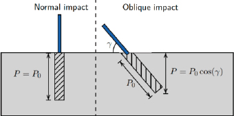
Fig. 6:
Schematic of normal and oblique impacts. The blue bar represents the projectile and the dashed bar represents the impact cavity.
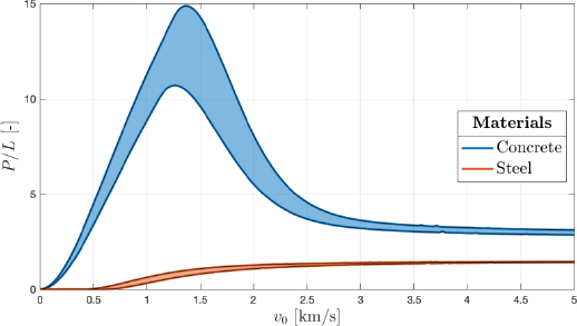
Fig. 7:
Normalised penetration depth graphed for concrete (blue) and steel (orange) and for a range of impact velocities v0.
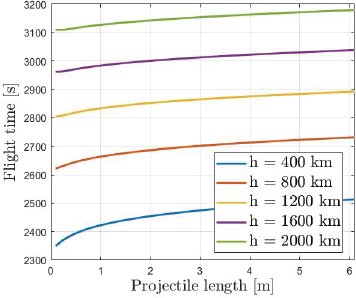
Fig. 8:
Flight time as a function of the projectile length for different altitudes.
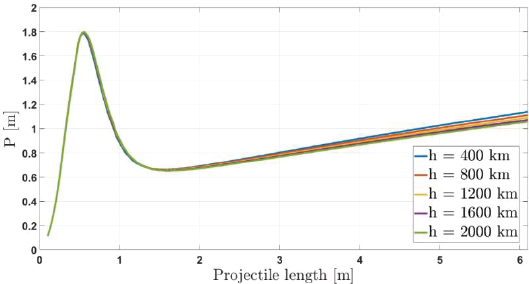
Fig. 9:
Penetration depth as a function of the projectile length for concrete targets.
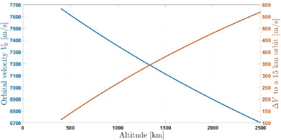
Fig. 10:
Initial orbital velocity and ΔV as a function of orbital height, necessary to transfer to a 15 km orbit.
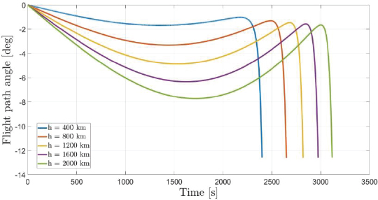
Fig. 11:
Flight path angle vs. time for a projectile length of 0.56 m for different start altitudes.
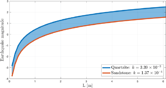
Fig. 12:
Earthquake magnitude for projectile lengths ranging from 0.1 m to 6.1 m.
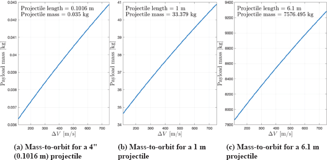
Fig. 13:
Mass-to-orbit per projectile for varied lengths of projectiles.
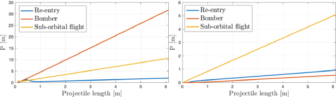
Fig. 14:
Penetration depth P for concrete and steel for different methods and projectile lengths. (Left: concrete; Right: steel).