
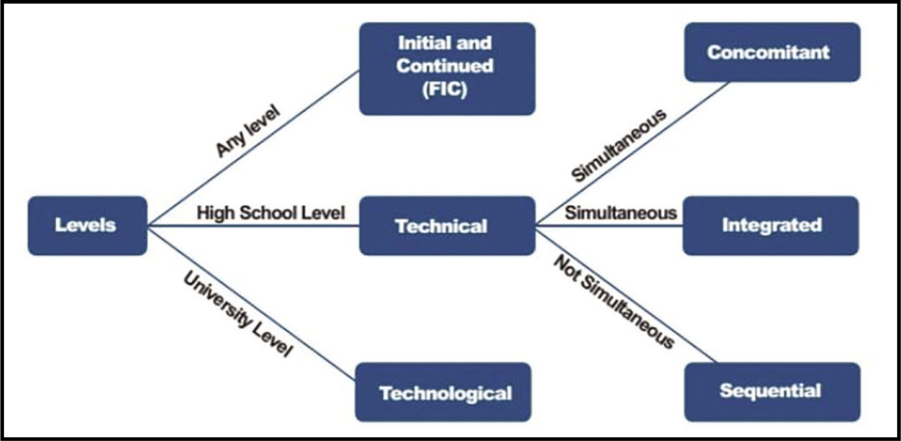
Figure 1
Types of Courses Tracks Offered Through PRONATEC [Amorim et al., 2015].
Table 1
Attrition
| Dep. Var.: | All Subsc. | Women | Men |
|---|---|---|---|
| Offer | −0.047 [0.043] | −0.057 [0.104] | −0.033 [0.048] |
| p–value | 0.267 | 0.585 | 0.489 |
| Number of observations | 1,444 | 467 | 977 |
[i] Notes: This table considers attrition in the full group of subscribers, and conditional on gender. Coefficients, standard errors and p-values are computed using specification (1), an ordinary least squares regression with course-by-site strata dummies and heteroskedasticity-robust standard errors [in brackets], using an indicator of not being in the endline sample as the dependent variable. Specification included control variables for sex, age, color and education.
Table 2
Within-Strata Balance Across Treatment Offer Arms, All Interviewed Subscribers
| (a) | (b) | (c) | (d) | (e) | |
|---|---|---|---|---|---|
| Mean (No offer) | Mean (Offer) | p−value (w. strata) | % Size | Number of obs. | |
| Male | 0.698 | 0.673 | 0.783 | −3.6% | 735 |
| Black, ’pardo’ or indigenous | 0.206 | 0.261 | 0.377 | 26.5% | 735 |
| Age | 27.25 (7.60) | 23.80 (6.46) | 0.949 | −12.7% | 735 |
| Mother completed high-school | 0.190 | 0.258 | 0.645 | 35.6% | 734 |
| Mother completed tertiary | 0.071 | 0.090 | 0.418 | 26.4% | 735 |
| Father completed high-school | 0.230 | 0.247 | 0.311 | 7.2% | 734 |
| Father completed tertiary | 0.048 | 0.061 | 0.944 | 27.6% | 735 |
| Concomitant modality | 0.246 | 0.473 | 0.072 | 92.2% | 735 |
| N | 126 | 609 | |||
| F–stat | p–value | ||||
| 0.838 | 0.569 |
[i] Notes: This table considers balancedness in the group of applicants surveyed at endline. Column (a) (column (b)) shows means and standard deviations (in parenthesis) for a pre-determined variable, for those not offered (offered) the opportunity to participate in the program with the scholarships in the schools and time frame considered. p-values in column (c) are computed for each variable using specification (1), an ordinary least squares regression with course-by-site strata dummies and heteroskedasticity-robust standard errors. Column (d) displays the unadjusted percent size of the raw difference between treatment offer arm means with respect to the control group mean, and column (e) shows the sample size. The last row shows the F-statistic and p-value from a regression of the treatment indicator on the full set of pre-determined variables and course-by-site strata dummies. Additional details on how the outcomes were created can be found in (see section “Definition of Main Variables” in Appendix).
Table 3
Within-Strata Balance Across Treatment Offer Arms, All Interviewed Subscribers by Gender Group
| Women | Men | |||||||||
|---|---|---|---|---|---|---|---|---|---|---|
| (a) | (b) | (c) | (d) | (e) | (a) | (b) | (c) | (d) | (e) | |
| Mean (No offer) | Mean (Offer) | p-value (w. strata) | % Size | Number of obs. | Mean (No offer) | Mean (Offer) | p-value (w. strata) | % Size | Number of obs. | |
| Black, “pardo” or indigenous | 0.184 | 0.256 | 0.189 | 39.1% | 237 | 0.216 | 0.263 | 0.829 | 22.0% | 498 |
| Age | 28.21 (8.24) | 22.71 (5.40) | 0.109 | 19.5% | 237 | 26.84 (7.32) | 24.33 (6.86) | 0.228 | −9.3% | 498 |
| Mother completed high-school | 0.184 | 0.256 | 0.909 | 39.1% | 237 | 0.193 | 0.259 | 0.774 | 34.2% | 497 |
| Mother completed tertiary | 0.053 | 0.095 | 0.974 | 81.4% | 237 | 0.080 (0.272) | 0.088 (0.283) | 0.304 | 10.4% | 498 |
| Father completed high-school | 0.211 | 0.266 | 0.373 | 26.5% | 237 | 0.239 | 0.237 | 0.506 | −0.6% | 497 |
| Father completed tertiary | 0.026 | 0.040 | 0.922 | 52.8% | 237 | 0.057 | 0.071 | 0.917 | 24.5% | 498 |
| Concomitant modality | 0.237 | 0.548 | 0.989 | 131.3% | 237 | 0.250 | 0.437 | 0.064 | 74.6% | 498 |
| N | 38 | 199 | 88 | 410 | ||||||
| F-stat | p-value | F-stat | p-value | |||||||
| 1.062 | 0.390 | 0.704 | 0.669 | |||||||
[i] Notes: This table considers balancedness in the group of female (leftmost columns) and male (rightmost columns) applicants surveyed at endline. Column (a) (column (b)) in each panel shows means and standard deviations (in parenthesis) for a pre-determined variable in a gender group, for those not offered (offered) the opportunity to participate in the program with the scholarships in the schools and time frame considered. p-values in column (c) are computed for each variable using specification (1), an ordinary least squares regression with course-by-site strata dummies and heteroskedasticity-robust standard errors, and p-values less than 0.15 are bolded. Column (d) displays the unadjusted percent size of the raw difference between treatment offer arm means with respect to the control group mean, and column (e) shows the sample size. The last row shows the F-statistic and p-value from a regression of the treatment indicator on the full set of pre-determined variables and course-by-site strata dummies. Additional details on how the outcomes were created can be found in (see section “Definition of Main Variables” in Appendix).
Table 4
Average Intent-to-treat Estimates on Technical and Non-Technical Education Graduation Rates
| Technical Education | General Education | |||||
|---|---|---|---|---|---|---|
| Dep. Var.: | (a) | (b) | (c) | (d) | (e) | (f) |
| Enrolled (PRONATEC) | Enrolled (any) | Graduated (PRONATEC) | Graduated (any) | Graduated High-school, concomitant | Enrolled (Tertiary) | |
| Panel A: All | ||||||
| Offer | 0.777 [0.030] | 0.641 [0.044] | 0.452 [0.041] | 0.234 [0.054] | 0.147 [0.068] | −0.034 [0.051] |
| No offer group mean | 0.016 | 0.198 | 0.087 | 0.437 | 0.774 | 0.389 |
| (i) p-value (H0: τITT) =0 | 0.000 | 0.000 | <0.001 | <0.001 | 0.031 | 0.513 |
| (ii) p-value (H0: τITT,i = 0, ∀ i) | 0.000 | 0.000 | <0.001 | <0.001 | 0.033 | 0.253 |
| Number of observations | 735 | 735 | 735 | 735 | 319 | 735 |
| Panel B: Women | ||||||
| Offer | 0.736 [0.055] | 0.596 [0.089] | 0.458 [0.070] | 0.200 [0.101] | 0.014 [0.074] | 0.016 [0.108] |
| No offer group mean | 0.026 | 0.211 | 0.053 | 0.368 | 0.889 | 0.447 |
| (i) p-value (H0: τITT) =0 | 0.000 | 0.000 | <0.001 | 0.050 | 0.845 | 0.884 |
| (ii) p-value (H0: τITT,i = 0, ∀ i) | 0.000 | 0.000 | <0.001 | 0.022 | 0.429 | 0.413 |
| Number of observations | 237 | 237 | 237 | 237 | 118 | 237 |
| Panel C: Men | ||||||
| Offer | 0.815 [0.034] | 0.678 [0.052] | 0.464 [0.051] | 0.238 [0.067] | 0.210 [0.088] | −0.018 [0.059] |
| No offer group mean | 0.011 | 0.193 | 0.102 | 0.466 | 0.727 | 0.364 |
| (i) p-value (H0: τITT) =0 | 0.000 | 0.000 | <0.001 | <0.001 | 0.018 | 0.756 |
| (ii) p-value (H0: τITT,i = 0, ∀ i) | 0.000 | 0.000 | <0.001 | <0.001 | 0.033 | 0.377 |
| Number of observations | 498 | 498 | 498 | 498 | 201 | 498 |
[i] Notes: This table considers the impact of the offer on technical and general education investments in the full sample of surveyed applicants (Panel A) and the sub-sample of female and male surveyed applicants (Panels B and C, respectively). All variables are self-reported and were collected from June to August of 2016 (an average of 2 years after the end of the program in our sample). Estimates are from the intent-to-treat specification (1), i.e., an ordinary least squares regression with course-by-site strata dummies, and standard errors computed using heteroskedasticity-robust standard errors are shown [in brackets]. Two p-values are displayed in the bottom rows for each panel: (i) two-tailed p-values for the null hypothesis of a zero average parameter H0: τITT = 0, using the reported standard errors; (ii) two-tailed randomization inference p-values for the sharp null hypothesis of no effect of the offer for any individual H0: τITT,i = 0, ∀ i, using 1,000 randomly drawn assignment vectors with fixed within-strata probabilities taken from the realized assignment. Additional information about the samples in each panel (no offer arm mean and sample size) can be found in the bottom rows and details on how the outcomes were created can be found in (see section “Definition of Main Variables” in Appendix).
Table 5
Average Intent-to-treat Estimates on Labor Market Outcomes
| Dep. Var.: | (a) | (b) | (c) | (d) | (e) | (f) |
|---|---|---|---|---|---|---|
| Employment | Labor market participation | Tenure | Formal employment | Work earnings | Wages (in logs) | |
| Panel A: All | ||||||
| PRONATEC Offer | 0.043 [0.042] | 0.053 [0.034] | 4.258 [4.486] | 0.051 [0.051] | 102.688 [108.5] | 0.046 [0.050] |
| No offer group mean | 0.802 | 0.865 | 33.008 | 0.690 | 1399.135 | 7.345 |
| (i) p-value (H0: τITT) =0 | 0.301 | 0.124 | 0.393 | 0.315 | 0.344 | 0.360 |
| (ii) p-value (H0: τITT,i = 0, ∀ i) | 0.270 | 0.102 | 0.345 | 0.309 | 0.312 | 0.399 |
| Number of observations | 735 | 735 | 726 | 735 | 731 | 567 |
| Panel B: Women | ||||||
| PRONATEC Offer | 0.217 [0.093] | 0.262 [0.078] | 16.410 [6.663] | 0.354 [0.097] | 513.000 [149.1] | 0.229 [0.101] |
| No offer group mean | 0.658 | 0.711 | 24.711 | 0.474 | 873.026 | 7.055 |
| (i) p-value (H0: τITT) =0 | 0.020 | 0.002 | 0.015 | <0.001 | 0.001 | 0.025 |
| (ii) p-value (H0: τITT,i = 0, ∀ i) | 0.008 | 0.000 | 0.011 | <0.001 | 0.001 | 0.018 |
| Number of observations | 237 | 237 | 235 | 237 | 237 | 166 |
| Panel C: Men | ||||||
| PRONATEC Offer | −0.017 [0.047] | −0.027 [0.035] | −0.542 [5.731] | −0.068 [0.058] | −39.420 [144.3] | −0.007 [0.060] |
| No offer group mean | 0.864 | 0.932 | 36.632 | 0.784 | 1626.318 | 7.445 |
| (i) p-value (H0: τITT) =0 | 0.717 | 0.416 | 0.736 | 0.252 | 0.899 | 0.810 |
| (ii) p-value (H0: τITT,i = 0, ∀ i) | 0.825 | 0.487 | 0.926 | 0.254 | 0.783 | 0.906 |
| Number of observations | 498 | 498 | 491 | 498 | 494 | 401 |
[i] Notes: This table considers the impact of the offer on labor market outcomes in the full sample of surveyed applicants (Panel A) and the sub-sample of female and male surveyed applicants (Panels B and C, respectively). All variables are self-reported and were collected from June to August of 2016 (an average of 2 years after the end of the program in our sample). Estimates are from the intent-to-treat specification (1), i.e., an ordinary least squares regression with course-by-site strata dummies, and standard errors computed using heteroskedasticity-robust standard errors are shown [in brackets]. Two p-values are displayed in the bottom rows for each panel: (i) two-tailed p-values for the null hypothesis of a zero average parameter H0: τITT = 0, using the reported standard errors; (ii) two-tailed randomization inference p-values for the sharp null hypothesis of no effect of the offer for any individual H0: τITT,i = 0, ∀ i, using 1,000 randomly drawn assignment vectors with fixed within-strata probabilities taken from the realized assignment. Additional information about the samples in each panel (no offer arm mean and sample size) can be found in the bottom rows and details on how the outcomes in columns (a)–(f) were created can be found in (see section “Definition of Main Variables” in Appendix).
Table 6
Average intent-to-treat Estimates on Standardized Indicators of Non-cognitive Skills
| Dep. Var.: | (a) | (b) | (c) | (d) | (e) | (f) | (g) |
|---|---|---|---|---|---|---|---|
| NC Index | Agreeableness | Conscientiousness | Extraversion | Neuroticism | Openness to experiences | Locus of control | |
| Panel A: All | |||||||
| Offer | 0.148 [0.141] | 0.062 [0.147] | 0.215 [0.143] | 0.182 [0.161] | 0.014 [0.146] | −0.030 [0.157] | −0.068 [0.157] |
| (i) p-value (H0: τITT) =0 | 0.296 | 0.673 | 0.133 | 0.258 | 0.924 | 0.847 | 0.664 |
| (ii) p-value (H0: τITT,i = 0, ∀ i) | 0.306 | 0.335 | 0.067 | 0.132 | 0.467 | 0.381 | 0.343 |
| Number of observations | 376 | 364 | 364 | 363 | 364 | 364 | 364 |
| Panel B: Women | |||||||
| Offer | 0.503 [0.183] | 0.360 [0.218] | 0.421 [0.241] | 0.690 [0.300] | 0.251 [0.262] | 0.284 [0.304] | −0.307 [0.283] |
| No offer group mean | −0.316 | −0.171 | −0.038 | −0.378 | −0.513 | −0.368 | 0.235 |
| (i) p-value (H0: τITT) =0 | 0.007 | 0.102 | 0.084 | 0.024 | 0.341 | 0.352 | 0.280 |
| (ii) p-value (H0: τITT,i = 0, ∀ i) | 0.028 | 0.089 | 0.066 | 0.009 | 0.188 | 0.205 | 0.138 |
| Number of observations | 111 | 106 | 106 | 105 | 106 | 106 | 106 |
| Panel C: Men | |||||||
| Offer | 0.0517 [0.188] | −0.002 [0.189] | 0.183 [0.181] | 0.062 [0.189] | −0.055 [0.187] | −0.082 [0.188] | 0.001 [0.195] |
| No offer group mean | 0.110 | 0.056 | 0.012 | 0.123 | 0.167 | 0.120 | −0.077 |
| (i) p-value (H0: τITT) =0 | 0.783 | 0.909 | 0.313 | 0.741 | 0.770 | 0.665 | 0.997 |
| (ii) p-value (H0: τITT,i = 0, ∀ i) | 0.761 | 0.466 | 0.138 | 0.403 | 0.401 | 0.354 | 0.474 |
| Number of observations | 265 | 258 | 258 | 258 | 258 | 258 | 258 |
[i] Notes: This table considers the impact of the offer on non-cognitive skills in the full sample of surveyed applicants (Panel A) and the sub-sample of female and male surveyed applicants (Panels B and C, respectively). All variables have been standardized with respect to the no offer group mean and standard deviation and were collected from June to August of 2016 (an average of 2 years after the end of the program in our sample). Estimates are from the intent-to-treat specification (1), i.e., an ordinary least squares regression with course-by-site strata dummies, and standard errors computed using heteroskedasticity-robust standard errors are shown in brackets. Heteroskedasticity-robust standard errors are in brackets, and two p-values are displayed in the bottom rows for each panel: (i) two-tailed p-values for the null hypothesis of a zero average parameter H0: τITT = 0, using the reported standard errors; (ii) two-tailed randomization inference p-values for the sharp null hypothesis of no effect of the offer for any individual H0: τITT,i = 0, ∀ i, using 1,000 randomly drawn assignment vectors with fixed within-strata probabilities taken from the realized assignment. Additional information about the samples in each panel (no offer arm mean and sample size) can be found in the bottom rows.
Table 7
Average intent-to-treat Estimates on Possible Channels Outcomes
| Possible Channels | ||||
|---|---|---|---|---|
| Dep. Var.: | (a) | (b) | (c) | (d) |
| NC Index | Ocupation (course area) | Certificate | Gateway | |
| Panel A: All | ||||
| Offer | 0.148 [0.141] | 0.175 [0.049] | 0.286 [0.079] | −0.017 [0.028] |
| No offer group mean | 0.165 | 0.270 | 0.059 | |
| (i) p-value (H0: τITT) =0 | 0.296 | 0.000 | 0.000 | 0.529 |
| (ii) p-value (H0: τITT,i = 0, ∀ i) | 0.306 | 0.001 | 0.000 | 0.467 |
| Number of observations | 376 | 571 | 587 | 569 |
| Panel B: Women | ||||
| Offer | 0.503 [0.183] | 0.079 [0.041] | 0.283 [0.201] | 0.015 [0.023] |
| No offer group mean | −0.316 | 0.043 | 0.250 | 0.000 |
| (i) p-value (H0: τITT) =0 | 0.007 | 0.054 | 0.160 | 0.503 |
| (ii) p-value (H0: τITT,i = 0, ∀ i) | 0.028 | 0.206 | 0.025 | 0.807 |
| Number of observations | 111 | 163 | 183 | 164 |
| Panel C: Men | ||||
| Offer | 0.052 [0.188] | 0.210 [0.064] | 0.283 [0.089] | −0.023 [0.037] |
| No offer group mean | 0.110 | 0.203 | 0.276 | 0.078 |
| (i) p-value (H0: τITT) =0 | 0.783 | 0.001 | 0.002 | 0.534 |
| (ii) p-value (H0: τITT,i = 0, ∀ i) | 0.761 | 0.003 | 0.000 | 0.539 |
| Number of observations | 265 | 408 | 404 | 405 |
[i] Notes: This table considers the impact of the offer on possible channels outcomes in the full sample of surveyed applicants (Panel A) and the sub-sample of female and male surveyed applicants (Panels B and C, respectively). All variables are self-reported and were collected from June to August of 2016 (an average of 2 years after the end of the program in our sample). Estimates are from the intent-to-treat specification (1), i.e., an ordinary least squares regression with course-by-site strata dummies, and standard errors computed using heteroskedasticity-robust standard errors are shown [in brackets]. Two p-values are displayed in the bottom rows for each panel: (i) two-tailed p-values for the null hypothesis of a zero average parameter H0: τITT = 0, using the reported standard errors; (ii) two-tailed randomization inference p-values for the sharp null hypothesis of no effect of the offer for any individual H0: τITT,i = 0, ∀ i, using 1,000 randomly drawn assignment vectors with fixed within-strata probabilities taken from the realized assignment. Additional information about the samples in each panel (no offer arm mean and sample size) can be found in the bottom rows and details on how the outcomes in columns (a)–(d) were created can be found in (see section “Definition of Main Variables” in Appendix).
Table 8
Average Intent-to-treat Estimates on Probability of being above Quantiles of Standardized Index of Non-cognitive Skills
| (a) | (b) | (c) | |
|---|---|---|---|
| All | Women | Men | |
| Probability of being above 20% | |||
| Offer | 0.0621 [0.0319] | 0.116 [0.0561] | 0.0446 [0.0384] |
| p-value (w. strata) | 0.052 | 0.038 | 0.246 |
| Probability of being above 40% | |||
| Offer | 0.0524 [0.0413] | 0.0652 [0.0779] | 0.0507 [0.0485] |
| p-value (w. strata) | 0.205 | 0.402 | 0.296 |
| Probability of being above 60% | |||
| Offer | 0.0224 [0.0461] | 0.0615 [0.0844] | 0.0228 [0.0548] |
| p-value (w. strata) | 0.627 | 0.466 | 0.678 |
| Probability of being above 80% | |||
| Offer | 0.0337 [0.0474] | −0.0655 [0.0871] | 0.0725 [0.0559] |
| p-value (w. strata) | 0.477 | 0.452 | 0.194 |
| P-value joint | 0.3442 | 0.0502 | 0.4181 |
| Number of observations | 735 | 237 | 498 |
[i] Notes: This table considers the impact of the offer on the probability of being above the 2nd, 4th, 6th and 8th deciles of the standardized non-cognitive index in the full sample of surveyed applicants (column (a)) and the sub-sample of female and male surveyed applicants (columns (b) and (c), respectively). The estimates are from simultaneous regressions of dummies for being above each decile on offer status, controls for color, age, gender and course-by-site strata dummies. Standard errors computed using heteroskedasticity-robust standard errors are shown [in brackets]. Two-tailed p-values for the null hypothesis of a zero average parameter H0: τITT = 0 are displayed in the bottom rows for each decile estimation. The p-value at the bottom of the table is for the null hypothesis that all coefficients are equal to zero.
Table 9
Possible Heterogeneos Effects
| (a) | (b) | (c) | |
|---|---|---|---|
| Dep. Var.: | Employment All | Employment Women | Employment Men |
| Offer | −0.000 [0.045] | 0.241 [0.111] | −0.099 [0.047] |
| p-value | 0.999 | 0.030 | 0.038 |
| Mother completed high-school | −0.242 [0.096] | −0.131 [0.220] | −0.292 [0.098] |
| p-value | 0.012 | 0.554 | 0.003 |
| Father completed high-school | 0.152 [0.105] | 0.046 [0.230] | 0.192 [0.111] |
| p-value | 0.149 | 0.841 | 0.084 |
| Offer*Mother completed high-school | −0.004 [0.092] | 0.064 [0.235] | −0.043 [0.092] |
| p-value | 0.968 | 0.785 | 0.643 |
| Offer*Father completed high-school | −0.009 [0.101] | −0.185 [0.247] | 0.090 [0.102] |
| p-value | 0.928 | 0.455 | 0.379 |
| Constant | 0.779 [0.093] | 0.373 [0.194] | 1.004 [0.099] |
| p-value | 0.000 | 0.056 | 0.000 |
| Number of observations | 735 | 237 | 498 |
[i] Notes: This table considers possible heterogeneous effects in the full group of subscribers, and conditional on gender. Coefficients, standard errors and p-values are computed using an ordinary least squares regression with course-by-site strata dummies and heteroskedasticity-robust standard errors [in brackets], using an indicator of being employed in the endline sample as the dependent variable. Specification included control variables for sex, age, and color. Parents’ educational level are used as a proxy for non-cognitive skills.
Table 10
OLS Estimates of the Correlation between the Treatment and Labor Market Outcomes
| (a) | (b) | |
|---|---|---|
| Dep. Var.: | Employment EEB | Employment PRONATEC |
| Treatment | 0.101 [0.077] | −0.007 [0.046] |
| p-value | 0.189 | 0.883 |
| Female | −0.228 [0.094] | −0.225 [0.092] |
| p-value | 0.016 | 0.015 |
| Age | −0.003 [0.017] | 0.001 [0.003] |
| p-value | 0.860 | 0.644 |
| Treatment*Female | 0.183 [0.118] | 0.158 [0.096] |
| p-value | 0.123 | 0.100 |
| Constant | 0.829 [0.345] | 0.780 [0.086] |
| p-value | 0.017 | 0.000 |
| Number of observations | 204 | 735 |
[i] Notes: This table considers correlation between attending a vocational course with no waiting list design (column (a)) or receiving an scholarship offer with a waiting list design (column (b)) and labor market outcomes. Specification in column (b) includes course-by-site strata dummies. Coefficients, standard errors and p-values are computed using an ordinary least squares regression with heteroskedasticity-robust standard errors [in brackets], using an indicator of being employed in the endline sample as the dependent variable. All specifications include control variables for sex and age.
Table 11
Structural Equation Model Parameters
| Dep. Var.: | (a) | (b) | (c) |
|---|---|---|---|
| All | Women | Men | |
| α1 | 0.801 [0.062] | 0.669 [0.125] | 0.875 [0.071] |
| p-value | 0.000 | 0.000 | 0.000 |
| β1 | 0.627 [0.086] | 0.800 [0.173] | 0.573 [0.100] |
| p-value | 0.000 | 0.000 | 0.000 |
| γ1 | 0.144 [0.102] | 0.964 [0.178] | −0.022 [0.124] |
| p-value | 0.160 | 0.000 | 0.862 |
| θ1 | 0.043 [0.039] | 0.034 [0.076] | −0.119 [0.045] |
| p-value | 0.266 | 0.652 | 0.007 |
| θ2 | 0.176 [0.003] | 0.477 [0.010] | 0.022 [0.003] |
| p-value | 0.000 | 0.000 | 0.000 |
| θ1* β1 | 0.029 | 0.129 | −0.086 |
| θ2* γ1 | 0.034 | 0.426 | 0.003 |
| θ1* β1 + θ2*γ1 | 0.063 | 0.556 | −0.082 |
| Number of observations | 364 | 107 | 257 |
[i] Notes: This table considers the impact of the offer on labor market outcomes through a structural equations model framework in the full sample of surveyed applicants (column (a)) and the sub-sample of female and male surveyed applicants (columns (b) and (c), respectively). The estimates are from simultaneous regressions of dummies for being enrolled and for graduating in PRONATEC, non-cognitive index and dummies for being employed. Controls for color, age, gender, mother education level and course-by-site strata dummies. Standard errors computed by delta method are shown [in brackets]. Two-tailed p-values for the null hypothesis of a zero average parameter H0: τITT = 0 are displayed in the bottom rows each parameter.
Table 12
Atrition (answered non-cognitive module), All Inter-viewed Subscribers and by Gender Group
| (a) | (b) | (c) | |
|---|---|---|---|
| All | Women | Men | |
| Answered | |||
| Offer | −0.015 [0.050] | 0.099 [0.090] | −0.058 [0.062] |
| p-value (w. strata) | 0.766 | 0.273 | 0.354 |
| Number of observations | 735 | 237 | 498 |
[i] Notes: This table considers attrition in the full group of subscribers, and conditional on gender. Coefficients, standard errors and p-values are computed using specification (1), an ordinary least squares regression with course-by-site strata dummies and heteroskedasticity-robust standard errors [in brackets], using an indicator of not answering the non-cognitive module as the dependent variable. Specification included control variables for sex, age and color.
Table 13
Within-Strata Balance Across Enrollment Arms, All Interviewed Subscribers who received an offer
| (a) | (b) | (c) | (d) | (e) | |
|---|---|---|---|---|---|
| Mean (No Enrollment) | Mean (Enrollment) | p-value (w. strata) | % Size | Number of obs. | |
| Male | 0.622 | 0.687 | 0.631 | 10.4% | 609 |
| Black, “pardo” or indigenous | 0.299 | 0.251 | 0.518 | −16.1% | 609 |
| Age | 23.559 | 23.867 | 0.461 | 1.3% | 609 |
| Mother completed high-school | 0.270 | 0.255 | 0.910 | −5.4% | 609 |
| Mother completed tertiary | 0.087 | 0.091 | 0.477 | 5.4% | 609 |
| Father completed high-school | 0.222 | 0.253 | 0.347 | 13.9% | 609 |
| Father completed tertiary | 0.055 | 0.062 | 0.507 | 12.9% | 609 |
| Concomitant modality | 0.457 | 0.477 | 0.0126 | 4.5% | 609 |
| N | 127 | 482 | |||
| F–stat | p–value | ||||
| 1.240 | 0.278 |
[i] Notes: This table considers balancedness in the group of applicants who received an scholarship offer surveyed at endline. Column (a) (column (b)) shows means and standard deviations (in parenthesis) for a pre-determined variable, for those not enrolled (enrolled) in the program with the scholarships in the schools and time frame considered. p-values in column (c) are computed for each variable using specification (1), an ordinary least squares regression with course-by-site strata dummies and heteroskedasticity-robust standard errors. Column (d) displays the unadjusted percent size of the raw difference between enrollment arm means with respect to the control group mean, and column (e) shows the sample size. The last row shows the F-statistic and p-value from a regression of the treatment indicator on the full set of pre-determined variables and course-by-site strata dummies. Additional details on how the outcomes were created can be found in (see section “Definition of Main Variables” in Appendix).
Table A1
LATE Estimates on Labor Market Outcomes
| Dep. Var.: | (a) | (b) | (c) | (d) | (e) | (f) |
|---|---|---|---|---|---|---|
| Employment | Labor market participation | Tenure | Formal employment | Work earnings | Wages (in logs) | |
| Panel A: All | ||||||
| Offer | 0.056 [0.053] | 0.068 [0.043] | 5.460 [5.613] | 0.066 [0.064] | 132.700 [136.9] | 0.058 [0.061] |
| No offer group mean | 0.802 | 0.865 | 33.008 | 0.690 | 1399.135 | 7.345 |
| p-value (H0: τITT) =0 | 0.291 | 0.112 | 0.331 | 0.304 | 0.332 | 0.344 |
| Number of observations | 735 | 735 | 726 | 735 | 731 | 567 |
| Panel B: Women | ||||||
| Offer | 0.295 [0.120] | 0.356 [0.104] | 22.31 [8.549] | 0.481 [0.129] | 697.3 [197.2] | 0.309 [0.131] |
| No offer group mean | 0.658 | 0.711 | 24.711 | 0.474 | 873.026 | 7.055 |
| p-value (H0: τITT) =0 | 0.014 | 0.001 | 0.009 | 0.000 | 0.000 | 0.018 |
| Number of observations | 237 | 237 | 235 | 237 | 237 | 166 |
| Panel C: Men | ||||||
| Offer | −0.021 [0.055] | −0.033 [0.041] | −0.661 [6.758] | −0.083 [0.068] | −48.630 [172.3] | −0.008 [0.069] |
| No offer group mean | 0.864 | 0.932 | 36.632 | 0.784 | 1626.318 | 7.445 |
| p-value (H0: τITT) =0 | 0.708 | 0.424 | 0.922 | 0.225 | 0.778 | 0.905 |
| Number of observations | 498 | 498 | 491 | 498 | 494 | 401 |
[i] Notes: This table considers the impact of participation on labor market outcomes in the full sample of surveyed applicants (Panel A) and the sub-sample of female and male surveyed applicants (Panels B and C, respectively). All variables are self-reported and were collected from June to August of 2016 (an average of 2 years after the end of the program in our sample). Estimates are from two-stage least squares regressions with course-by-site strata dummies, and standard errors computed using heteroskedasticity-robust standard errors [in brackets]. Additional information about the samples in each panel (no offer arm mean, p-values and sample size) can be found in the bottom rows and details on how the outcomes were created can be found in Appendix 7.
Table A2
LATE Estimates on Standardized Indicators of Non-cognitive Skills
| Dep. Var.: | (a) | (b) | (c) | (d) | (e) | (f) | (g) |
|---|---|---|---|---|---|---|---|
| NC Index | Agreeableness | Conscientiousness | Extraversion | Neuroticism | Openness to experiences | Locus of control | |
| Panel A: All | |||||||
| Offer | 0.187 [0.172] | 0.132 [0.177] | 0.250 [0.169] | 0.253 [0.187] | 0.057 [0.177] | −0.022 [0.189] | −0.071 [0.185] |
| p-value (H0: τITT) =0 | 0.277 | 0.458 | 0.139 | 0.176 | 0.749 | 0.909 | 0.703 |
| Number of observations | 376 | 376 | 376 | 376 | 376 | 376 | 376 |
| Panel B: Women | |||||||
| Offer | 0.697 [0.240] | 0.590 [0.277] | 0.548 [0.294] | 0.856 [0.334] | 0.279 [0.327] | 0.444 [0.350] | −0.468 [0.344] |
| No offer group mean | −0.316 | −0.171 | −0.038 | −0.378 | −0.513 | −0.368 | 0.235 |
| p-value (H0: τITT) =0 | 0.004 | 0.033 | 0.062 | 0.011 | 0.394 | 0.205 | 0.174 |
| Number of observations | 111 | 111 | 111 | 111 | 111 | 111 | 111 |
| Panel C: Men | |||||||
| Offer | 0.060 [0.207] | 0.007 [0.208] | 0.176 [0.197] | 0.108 [0.205] | 0.000 [0.210] | −0.085 [0.210] | 0.047 [0.212] |
| No offer group mean | 0.110 | 0.056 | 0.012 | 0.123 | 0.167 | 0.120 | −0.077 |
| p-value (H0: τITT) =0 | 0.771 | 0.975 | 0.371 | 0.598 | 1.000 | 0.684 | 0.827 |
| Number of observations | 265 | 265 | 265 | 265 | 265 | 265 | 265 |
[i] Notes: This table considers the impact of participation on non-cognitive skills outcomes in the full sample of surveyed applicants (Panel A) and the sub-sample of female and male surveyed applicants (Panels B and C, respectively). All variables are self-reported and were collected from June to August of 2016 (an average of 2 years after the end of the program in our sample). Estimates are from two-stage least squares regressions with course-by-site strata dummies, and standard errors computed using heteroskedasticity-robust standard errors [in brackets]. Additional information about the samples in each panel (no offer arm mean, p-values and sample size) can be found in the bottom rows and details on how the outcomes were created can be found in Appendix 7.
Table A3
LATE Estimates on Possible Channels Outcomes
| Possible Channels | ||||
|---|---|---|---|---|
| Dep. Var.: | (a) | (b) | (c) | (d) |
| NC Index | Ocupation (course area) | Certificate | Gateway | |
| Panel A: All | ||||
| Offer | 0.187 [0.172] | 0.217 [0.058] | 0.334 [0.090] | −0.022 [0.034] |
| 0.277 | 0.000 | 0.000 | 0.515 | |
| No offer group mean | 0.165 | 0.270 | 0.059 | |
| p-value (H0: τITT) =0 | 0.296 | 0.000 | 0.000 | 0.529 |
| Number of observations | 376 | 571 | 587 | 569 |
| Panel B: Women | ||||
| Offer | 0.697 [0.240] | 0.108 [0.050] | 0.318 [0.205] | 0.020 [0.028] |
| 0.004 | 0.032 | 0.121 | 0.465 | |
| No offer group mean | −0.316 | 0.043 | 0.250 | 0.000 |
| p-value (H0: τITT) =0 | 0.007 | 0.054 | 0.160 | 0.503 |
| Number of observations | 111 | 163 | 183 | 164 |
| Panel C: Men | ||||
| Offer | 0.060 [0.207] | 0.247 [0.072] | 0.32 [0.093] | −0.027 [0.042] |
| 0.771 | 0.001 | 0.001 | 0.517 | |
| No offer group mean | 0.110 | 0.203 | 0.276 | 0.078 |
| p-value (H0: τITT) =0 | 0.783 | 0.001 | 0.002 | 0.534 |
| Number of observations | 265 | 408 | 404 | 405 |
[i] Notes: This table considers the impact of participation on possible channels outcomes in the full sample of surveyed applicants (Panel A) and the sub-sample of female and male surveyed applicants (Panels B and C, respectively). All variables are self-reported and were collected from June to August of 2016 (an average of 2 years after the end of the program in our sample). Estimates are from two-stage least squares regressions with course-by-site strata dummies, and standard errors computed using heteroskedasticity-robust standard errors [in brackets]. Additional information about the samples in each panel (no offer arm mean, p-values and sample size) can be found in the bottom rows and details on how the outcomes were created can be found in Appendix 7.
Table A4
Number of subscriptions by municipality and course
| Course | Chapecó | Itapiranga | S. M. Oeste | Xanxerê | Total |
|---|---|---|---|---|---|
| Mechanics | 201 | 0 | 0 | 77 | 278 |
| Administration | 8 | 0 | 0 | 0 | 8 |
| Pharmaceutical | 0 | 0 | 5 | 0 | 5 |
| Computer Network | 163 | 49 | 30 | 38 | 280 |
| Workplace Safety | 223 | 0 | 28 | 42 | 293 |
| Building | 31 | 0 | 0 | 0 | 31 |
| Electrotechnology | 113 | 76 | 35 | 0 | 224 |
| Electronics | 46 | 0 | 0 | 0 | 46 |
| Electromechanics | 0 | 0 | 62 | 61 | 123 |
| Food Technology | 92 | 0 | 64 | 0 | 156 |
| Total | 877 | 125 | 224 | 218 | 1,444 |
[i] Source: author's elaboration using survey and administrative data.