
1. Introduction
Achieving gender equality and empowerment of all women and girls is one of the 17 sustainable development goals of the United Nation. Beliefs about women's roles in society or the home often make achieving these goals challenging. Despite how entrenched beliefs about gender may be today, evidence suggests that beliefs may partially be a cultural by-product of idiosyncratic historical conditions. For example, the historical reliance on plow agriculture may have caused women to specialize in household production (Alesina et al., 2013), or reliance on pastoralism may have led some societies to develop practices to restrict women's sexuality (Becker, 2019). This raises the following question – can this process work in reverse? In other words, can external conditions or shocks also cause gender norms to erode? Can societies unlearn gender roles through even temporary experiences with more-equitable roles? Motivated by these questions, our paper studies whether temporary migration spells of husbands in rural Nepal leads couples to permanently adopt more-equitable norms in decision-making. Importantly, we also study the economic consequences of this shift in decision-making.
We use panel data on rural Nepali households to study how a husband's migration interacts with intrahousehold decision-making power and expenditure decisions within households over time. We show that during migration spells, decision-making power (both sole and joint) shifts from a husband to his wife. The shift is large and represents 10% of total decisions. In the Nepali context, this is not an a priori obvious result – Nepali married couples often live with the husband's parents, who typically command some authority in the household and could easily step in for their son upon his leave. Moreover, while husbands are migrating, they still report exerting some control over decisions, suggesting that this is not merely mechanical.
When decisions shift to the wife, we provide evidence that households decrease their spending on temptation goods (alcohol and tobacco products) by 105–120%. We provide some evidence that this reduction is offset by increased spending on children's education and clothing, although we interpret those results with some caution. Insofar as these reallocations are caused by the shift in decision-making power, this demonstrates how altering gender roles in decision-making could have meaningful economic impacts on developing countries.
Of course, such a change in spending habits could easily be attributed to an income effect. Higher wages motivate migration, and labor market or migration frictions likely mean that substantial wage arbitrage opportunities persist across locations. Naturally, we find that migration spells increase household income. To assess whether the spending changes are attributable to an income effect or changes in decision-making power, we exploit the fact that many households allow their sons to migrate. Although sending sons for migrant work increases household income, we do not observe changes in decision-making power or shifts in expenditures similar to the ones when husbands migrate. This suggests that the shifts in expenditures that occur when husbands migrate is specific to the migration of a husband (a primary household decision-maker) rather than income effects induced by migration spells in general. In other words, decision-making appears to be the channel that mediates the changes in expenditures that we observe.
Women's decision-making power is a key component of women's economic empowerment. Kabeer (1999) defines empowerment as the process by which people expand their ability to make strategic life choices, particularly in contexts in which this ability had been denied to them. Therefore, decision-making power is an important outcome in and of itself: if male migration triggers women's participation in household decision-making, then women's empowerment could be an important welfare implication of migration.
Moreover, decision-making may mediate other outcomes, such as how the household spends money. If women gain meaningful decision-making power, then assuming the husband and wife do not share identical preferences, we also expect changes in household economic decisions. In fact, many programs target female beneficiaries based on an expectation that women prefer to invest more in children (Duflo, 2012; Handa, 1996; Hoddinott and Haddad, 1995; Thomas, 1990), and specifically girls (Duflo, 2003; Qian, 2008; Thomas, 1990, 1994). Along these lines, several studies have demonstrated increased investment in children's education following migration (Antman, 2011, 2012; Edwards and Ureta, 2003; Yang, 2008),1 with some evidence that these investments are related not only to the alleviation of cash constraints made possible through remittances but also to women's preferences. For example, Cortes (2015) shows that the migration of a mother (rather than a father) has a negative impact on children's’ educational attainment, likely due to lower parental time inputs. Such child investments have obvious implications on households’ welfare and downstream ability to grow out of poverty. Even if these are short-lived effects and are terminated at the end of a migration spell, child investments in health or education that occur at key points in a child's development can have long-term impacts (Blattman et al., 2018).
Our work lies at the intersection of literature on gender and migration. Much of the work at this intersection studies how female migration interacts with women's agency and gender inequality (e.g., Hughes, 2019; Parrado et al., 2005; Stecklov et al., 2010; Sultana and Fatima, 2017). Our results specifically contribute to a growing literature studying how migration affects household decision-making among female family members left behind. Clemens and Tiongson (2017) exploit a natural experiment and use a regression discontinuity design to show that when household members migrate from the Philippines to Korea, women take on greater responsibility for household decisions. Furthermore, they spend more on education, health, and quality-of-life goods (e.g., ceremonies); they also borrow less, save more, and are more likely to send children to private school and visit private clinics. They present suggestive evidence that these effects work through not only remittances but a change in household decision-making power. Antman (2015) finds a similar pattern in Mexico: decision-making power shifts in favor of the spouse left behind during a migration spell, and the household tendency to devote a larger share of resources to girls rather than boys during this period. In contrast to these findings, Göbel (2013) finds no evidence of differences in how female- and male-headed households spend remittances that their migrant spouses send home. Other work has highlighted that geographic separation could introduce asymmetric information about household decisions, therefore allowing the wife to make de facto independent decisions about the household budget (Chen, 2013; Ambler, 2015; Ashraf et al., 2015).
A concern in interpreting our results is that migration is not a randomly assigned event: households select into migration. Moreover, this decision may be correlated with other factors that also affect household decision-making or finances. For example, one concern may be that households selecting into migration are more likely to see changes in decision-making power, i.e., migrant households are more open to adopting more-equitable norms. Past work suggests that, if anything, the bias goes the opposite way. Nobles and McKelvey (2015) find that when women are more in control of household resources, husbands are less likely to migrate. This suggests that households in which the husband migrates are not likely to be the type of households in which women's empowerment grows over time; in fact, they may be the opposite type of household, thus working against our results.
We address these issues in several ways. Similar to Antman (2015), our main empirical approach uses household fixed effects (FE) and thus compares households to themselves over time as the husband's migration status changes. This approach controls for any unobserved time-invariant differences among households. Selection into migration – likely on the basis of youth, earnings potential, risk tolerance, or other unobservables that could easily affect our outcomes – will be controlled for by these FE. Moreover, we include a specification whereby we limit our sample to households in which the husband migrates at some point, therefore conditioning on selection into current/eventual migration (so only selection into the timing of migration spells remains as a confounder). Lastly, we include household-specific time trends to control for unobserved time-varying factors, such as differential trends in consumption. While our estimates rely on several assumptions, we argue that our empirical approach controls for the factors that most plausibly threaten our interpretation. Finally, we argue that the narrative as a whole provides a compelling case that our results are not simply spurious.
Our novel contribution to this literature is to highlight the potential for persistence of these effects (which past work has not studied) and to offer an explanation for this. We explore persistence by identifying asymmetries in the magnitude of behavioral changes when the husband leaves vs. when he returns. This decomposition allows us to see whether decisions return to their original, premigration-spell trend on the husband's return. Following a migrant's return, we find suggestive evidence that husbands resume their role in economic decisions, but decisions are more likely to be made jointly. Despite this, expenditures appear to return to premigration levels, which suggests that women may lack bargaining power when making joint decisions. Nevertheless, a lasting change in who participates in decisions is an important first step toward more equality in decision-making. This finding underscores the potential role of temporary migration spells in triggering lasting cultural change around gender norms.
We show how these persistent effects can be explained by a habit-formation model (e.g., Becker and Murphy, 1998). Migration disrupts the household's usual decision-making process, which necessitates that the household form new habits. During this time, the household “learns by doing” – e.g., couples may realize that women are indeed capable of making financial decisions. Preferences slowly change over who makes decisions, and the new habit of more-equitable decision-making starts to stick. The longer a migrant stays away, the more likely this habit forms. Consistent with this narrative, we find that the contemporaneous changes in decision-making power are concentrated in households that experience longer (at least 6 months) migration spells. This result helps rule out an alternative explanation for persistence – that migrants “bring home” norms or ideas from the country they visit (Batista and Vicente, 2011; Beine and Sekkat, 2013; Bertoli and Marchetta, 2015; Böhme, 2015; Lodigiani and Salomone, 2020).2 Given the prevalence of seasonal migration in developing countries, our findings suggest that even temporary migration could have important consequences for women's empowerment.
Identifying the habit-formation mechanism broadens the policy impact of our paper by illustrating how exactly could policies be designed to improve women's empowerment. This contributes to a growing literature studying how policies can be effectively designed to change pervasive gender norms. For example, correcting individual beliefs about others’ privately held beliefs on gender may lead to less distortion of female labor supply in Saudi Arabia (Bursztyn et al., 2020). Similarly, giving women individual bank accounts, therefore incentivizing them to work, may indirectly change gender norms (Field et al., 2021). Our work suggests a new mechanism that policies aimed at similar goals could apply: promoting learning and habit formation through a temporary disruption in the decision-making process may facilitate long-term cultural change.
The remainder of the paper is organized as follows. We begin, in Section 2, with a description of the unique Nepali context and our data, which underscores the policy relevance of our analysis. In Section 3, we present our main empirical strategy and discuss our identifying assumptions. Results are presented in Section 4. In Section 5, we discuss how our results can be explained by a model of habit formation. We close in Section 6 with some concluding remarks.
2. Data and Background
The relationship between migration and gender norms is of considerable interest in Nepal and throughout much of South Asia. In 2015, remittances made up >30% of Nepali gross domestic product (GDP) – a share considerably higher than in most countries (World Bank Group, 2018). As a South Asian country, Nepal is home to gender norms that often constrain women's opportunities in the labor market, education, or autonomy over decisions (Asian Development Bank [ADB], 2010).3,4 Although recognized as having made progress in recent years, Nepali women are still considerably disadvantaged relative to men, and patriarchal social norms still dictate women's role in society (Khanal, 2018; Holmelin, 2019).
Our main data source is the “Heifer Nepal Smallholders in Livestock Value Chain” impact evaluation panel survey data collected in 2014, 2016, 2017, and 2018 from rural Nepali households residing in communities across seven districts (see Figure A1 in the Appendix for a map). In each round of the survey, female respondents were asked about household demographics and finances, economic activity including migration status of household members, and economic decision-making. We include only those households in which a married, female respondent was interviewed in the first round and at least one other time. Our full sample is an unbalanced panel of 2,508 households.4
The survey data were collected for the evaluation of a livestock transfer program. Details of the randomized program evaluation process are provided by Janzen, et al. (2018). One concern may be that this program affected migration, leading us to conflate migration spells with program treatment effects. However, the treatment is not correlated with the decision to migrate, mitigating this concern.5 A second concern is that our results may be concentrated among households in the treatment group, therefore reflecting interaction effects between the livestock transfer program and migration. The existence of an interaction effect would not necessarily be surprising: Janzen et al. (2018) provide evidence that the livestock transfer program increased women's empowerment, and it seems plausible that a highly empowered woman is more likely to gain decision-making power when her husband migrates, as well as retain that power when he returns. Yet, this would be true of any empowering program globally. The concern would be much more problematic if there was something unique about this particular development program that allows it to interact with migration in ways that would not replicate elsewhere. Instead, the program is a fairly typical livestock development program and probably not that different from other rural agricultural contexts globally in which livestock or other agricultural development projects are constantly being implemented. To further alleviate these concerns, we estimate all specifications with and without the inclusion of (randomized) treatment dummy variables and treatment interaction terms. The results are robust.6 All things considered, it does not seem plausible that the livestock transfer program poses a significant threat to how we interpret our results.
2.1. Migration
In 2017–2018, remittances made up nearly 28% of sample households’ income, highlighting the extent to which many families in our sample depend on migrant work.7 Migration spells occur frequently: households have 1.5 migrants on average, and 53% of households have at least one migrant over the course of four interviews (spanning 5 years). Representative statistics from the nationally representative 2016 Demographic and Health Survey (DHS) survey suggest that our sample may disproportionately pull from villages with higher migration rates (Ministry of Health, 2017).8
Migrants are defined as household members not currently residing at home. Data from the final three survey rounds indicates that 96% of husbands not currently residing at home listed “migrated for work” as their purpose for leaving, suggesting that this is a good indicator of migration.9 Husbands who migrate are likely to have a destination outside of Nepal (76%) or be away for >6 months (83%). While we do not have detailed information on destination countries,10 male migrants with a destination outside of Nepal in the 2016 DHS sample were likely to migrate to the Middle East (32%) or India (17%) (Ministry of Health, 2017).
Table 1 provides further context by illustrating what sorts of characteristics correlate with the decision to migrate. We report the overall sample mean and then disaggregate means by whether the husband has migrated at least once during the observed periods (“ever migrate”) or not (“never migrate”). Migrant husbands are younger, more educated, and more likely to be literate than husbands who are not observed as migrants at any time in the data. Similarly, the wives of migrant men are younger, more educated, and more likely to be literate than wives of husbands who remain at home. These differences highlight the importance of an empirical strategy that controls for selection into migration or, more broadly, differences between migrant and nonmigrant households.
Table 1
Characteristics by migrant status
| (1) | (2) | (3) | (4) | |
|---|---|---|---|---|
| Overall | Ever migrate | Never migrate | P-value (2) = (3) | |
| Panel A | ||||
| Husband characteristics | ||||
| Age | 46.119 | 38.934 | 50.720 | 0.000*** |
| [12.921] | [9.339] | [12.800] | ||
| Years of education | 5.104 | 6.219 | 4.391 | 0.000*** |
| [3.940] | [3.517] | [4.030] | ||
| Can read or write | 0.763 | 0.877 | 0.690 | 0.000*** |
| [0.365] | [0.270] | [0.398] | ||
| Wife characteristics | ||||
| Age | 41.650 | 35.076 | 45.859 | 0.000*** |
| [12.143] | [9.016] | [12.020] | ||
| Years of education | 2.513 | 3.770 | 1.708 | 0.000*** |
| [3.545] | [3.790] | [3.125] | ||
| Can read or write | 0.527 | 0.677 | 0.431 | 0.000*** |
| [0.401] | [0.369] | [0.391] | ||
| N | 2,508 | 979 | 1,529 | 2,508 |
| Panel B | ||||
| Household characteristics | ||||
| No. of resident household members | 3.483 | 3.629 | 3.386 | 0.000*** |
| [1.854] | [1.745] | [1.916] | ||
| Resident mother-in-law | 0.230 | 0.316 | 0.174 | 0.000*** |
| [0.421] | [0.465] | [0.379] | ||
| Resident father-in-law | 0.159 | 0.232 | 0.110 | 0.000*** |
| [0.365] | [0.422] | [0.313] | ||
| Resident daughter-in-law | 0.185 | 0.084 | 0.251 | 0.000*** |
| [0.388] | [0.277] | [0.434] | ||
| Shocks | ||||
| Natural disaster (nonearthquake) | 0.044 | 0.039 | 0.047 | 0.092* |
| [0.206] | [0.194] | [0.213] | ||
| Serious illness | 0.223 | 0.213 | 0.230 | 0.074* |
| [0.416] | [0.409] | [0.421] | ||
| Death of household member | 0.055 | 0.053 | 0.056 | 0.630 |
| [0.228] | [0.225] | [0.230] | ||
| Falling agricultural prices | 0.131 | 0.109 | 0.146 | 0.000*** |
| [0.338] | [0.312] | [0.353] | ||
| Decrease in income | 0.155 | 0.134 | 0.170 | 0.000*** |
| [0.362] | [0.341] | [0.375] | ||
| Loss of employment | 0.023 | 0.020 | 0.025 | 0.178 |
| [0.151] | [0.141] | [0.156] | ||
| Mercalli scale 2015 earthquake | 6.926 | 6.870 | 6.962 | 0.000*** |
| [0.505] | [0.525] | [0.488] | ||
| N | 7,572 | 3,013 | 4,559 | 7,572 |
[i] Notes: This table reports mean values with standard deviations in brackets. Column 1 includes all households, Column 2 is limited to households in which the husband migrates at some point, and Column 3 is limited to households in which the husband has not reported migrating during any survey round. Column 4 reports the p-value for a t-test of differences between columns 2 and 3. In panel A, data are at the household level and characteristics are defined using the mean over time (2014–2018) for each household. Data in panel B are pooled 2014–2018 values. The nonearthquake shock averages represent the fraction of households that experienced a given event (e.g., death of a household member) since the previous round of data were collected.
Given that migrants are younger on average than those who do not migrate, it is unsurprising that migrants are also more likely to have a resident mother-in-law or father in-law. Households with recent migrants are mechanically younger; so, likewise, it is unsurprising that they are more likely to be in joint households than future/current migrants. Joint households, where young couples live with the husband's parents, are common in Nepal. Qualitative research has shown that joint households in South Asian contexts are typically headed first by the father-in-law, or in the case of his absence – his wife, their son, and finally, the son's wife (e.g., Bloom et al., 2001). This highlights the theoretical ambiguity of the impact of a husband's migration on his wife's decision-making power, since men may easily transfer decision-making power to their parents rather than their wives.
Negative economic shocks could push individuals to migrate (Shrestha, 2017) or could prevent individuals from migrating if doing so requires investment or resources. Importantly, we have indicators for whether the household experienced a natural disaster, serious illness of a household member, death of a household member, falling agricultural prices, decrease in income, or loss of employment since the previous survey round. In addition to these shocks, we also have information about the severity of the 7.8-magnitude earthquake that hit Nepal on April 25, 2015. We use geospatial data from the United States Geological Survey's (USGS) Earthquake Hazards Program to construct a measure of the earthquake intensity at the village development committee (VDC) level.11 In general, households in which the husband migrates tend to experience less shocks on average, consistent with the idea that migration may require significant resources or investment. We will control for all observed shocks in our analysis. The next few sections describe the outcome variables used in our analysis. Table 2 reports these outcomes broken up by ever-migrant status.
Table 2
Outcomes by migrant status
| (1) | (2) | (3) | (4) | |
|---|---|---|---|---|
| Overall | Ever migrate | Never migrate | P-value (2) = (3) | |
| Panel A: Decision-making over all categories | ||||
| Husband alone | 0.136 | 0.105 | 0.156 | 0.000*** |
| [0.209] | [0.187] | [0.220] | ||
| Husband and wife jointly | 0.338 | 0.304 | 0.361 | 0.000*** |
| [0.313] | [0.313] | [0.310] | ||
| Wife alone | 0.108 | 0.177 | 0.062 | 0.000*** |
| [0.208] | [0.256] | [0.152] | ||
| Panel B: Income and financial behavior | ||||
| Annual income | 11.562 | 11.826 | 11.388 | 0.000*** |
| [3.117] | [2.931] | [3.223] | ||
| Savings deposited in past month | 4.425 | 4.699 | 4.244 | 0.000*** |
| [3.056] | [3.036] | [3.055] | ||
| Currently borrowing | 6.922 | 7.049 | 6.838 | 0.128 |
| [5.886] | [5.855] | [5.906] | ||
| Currently lent | 1.630 | 1.945 | 1.421 | 0.000*** |
| [4.006] | [4.307] | [3.780] | ||
| Panel C: Expenditures | ||||
| Temptation goods | 4.124 | 3.528 | 4.515 | 0.000*** |
| [3.685] | [3.677] | [3.638] | ||
| Health care | 5.971 | 5.765 | 6.107 | 0.000*** |
| [3.404] | [3.428] | [3.381] | ||
| Ceremonies or celebrations | 7.111 | 7.063 | 7.143 | 0.143 |
| [2.298] | [2.357] | [2.259] | ||
| Child education | 5.128 | 5.856 | 4.641 | 0.000*** |
| [3.381] | [2.961] | [3.553] | ||
| Child clothing | 5.184 | 5.860 | 4.730 | 0.000*** |
| [2.985] | [2.518] | [3.181] | ||
| Adult women clothing | 6.330 | 6.424 | 6.268 | 0.000*** |
| [1.626] | [1.464] | [1.721] | ||
| N | 7,572 | 3,013 | 4,559 | 7,572 |
[i] Notes: This table reports mean values with standard deviations in brackets. Column 1 includes all households, Column 2 is limited to households in which the husband migrates at some point, and Column 3 is limited to households in which the husband has not reported migrating during any survey round. Column 4 reports the p-value for a t-test of differences between columns 2 and 3. The data are at the household level and are pooled 2014–2018 values. Decision-making variables are the fractions of decisions over which the decision-making power is distributed as described out of all categories included in the analysis: temptation goods, health care, ceremonies, children's education, children's clothing, and adult women's clothing. See Section C of the Appendix for more details on how these variables are composed. All rupee amounts are transformed by the inverse hyperbolic sine.
2.2. Decision-making
Our decision-making data are based on a survey question (posed to the wife) that asks who in the household makes the decision regarding a particular expenditure. We first create variables for each good that describe who makes the decision – the husband alone, wife alone, or husband and wife jointly.12 Then, we take the average of the indicators across goods within each category; the final variable represents the fraction of goods within a category over which the husband, the wife, or both have control. Expenditure categories include temptation goods (alcohol and tobacco), formal health care, ceremonies and celebrations, children's education, children's clothing, and adult women's clothing.13
Across all households in our sample, 34% of expenditure decisions are made jointly, while men alone decide 14% and their wives alone decide 11%. But, averaging across households hides substantial heterogeneity by the husband's migrant status. Figure 1 reveals a striking pattern that illustrates the main narrative of our empirical results. Before husbands migrate, 27% of decisions are made jointly, while 18% are made by the husband alone and 11% are made by the wife alone.
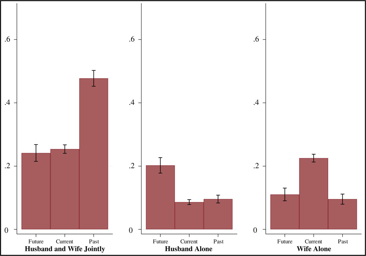
Figure 1
Fraction of decisions made jointly/alone across husband's migration status.
Data are pooled 2014–2018 values. The figure depicts the mean fraction of all expenditure decisions (considered in this paper) that are made either by the individual or jointly as indicated; 95% confidence intervals are also displayed. See Section C1 of the Appendix for more details on how each expenditure category is constructed. “Future” indicates that the husband will migrate in the next period, “current” indicates migration in the current period, “past” indicates that the husband migrated in the previous period, and “never” indicates that the husband did not migrate during any of the survey rounds. These groups are mutually exclusive and, therefore, we omit the 102 observations that both migrated in the previous period and will migrate in the future period.
During migration spells, decision-making power shifts in favor of the wife as she becomes more than twice as likely as before to make sole decisions. Although she is unlikely to retain newly acquired sole decision-making power following her husband's return, a much higher share of subsequent decisions (47%) are made jointly. This anticipates our main finding: a husband's migration spell seems to increase his wife's involvement in household decision-making, which she partially retains upon his return. Moreover, these summary statistics highlight why decision-making is not simply mechanically related to migration status – clearly, husbands remain involved to some extent upon migrating.
2.3. Finances
Household finances undoubtedly play a role in a household's decision to migrate and also likely change as a result of migration, which explains why much of the existing literature on the welfare effects of migration has primarily focused on how remittances or incomes affect households. For example, Yang (2008) takes advantage of a unique natural experiment, using plausibly exogenous exchange rate fluctuations, to show that remittances lead to increased investment in the Philippines. Bryan et al. (2014) apply a randomized incentive to show increased food and nonfood expenditures among migrant households in Bangladesh. Gibson et al. (2017) use a difference-in-differences approach to demonstrate increased income, consumption, and savings among migrant households in Tonga. Yang (2011) and Adams (2011) provide thorough summaries of this literature.
Acknowledging this important income channel, we apply data on annual household income, savings deposited in the past month, amount borrowed currently, and amount lending currently (to capture informal lending). Throughout the analysis, any monetary values are in 2014 Nepali rupees (adjusted for inflation) and transformed using the inverse hyperbolic sine (asinh).14
2.4. Expenditures
Mirroring the construction of decision-making categories, we observe spending on six categories of goods: temptation goods (alcohol and tobacco), formal health care, ceremonies and celebrations, children's education, children's clothing, and adult women's clothing. As with the financial data, throughout the analysis, amounts are in 2014 Nepali rupees (adjusted for inflation) and transformed using the inverse hyperbolic sine (asinh). The survey asked the respondent to recall the expenditure amounts in varying time horizons; hence, we harmonize the amount when applicable (e.g., yearly expenditures are divided by 12). See Appendix (Section C1) for an explanation of how the items are aggregated.15
3. Empirical Strategy
The key empirical challenge for this analysis is that the decision to migrate is not randomly assigned. It therefore may be correlated with factors that also affect the outcomes, resulting in an issue of omitted variables. Moreover, many variables that factor into one's decision to migrate (such as earnings potential) are fundamentally unobserved. To overcome this challenge, similar to Antman (2015), we use household FE to compare changes in the outcomes within households over time as the husband's migration status changes. Put differently, this approach estimates the average change in the outcomes that households experience when the husband migrates, while holding constant all fixed household characteristics that may correlate with both migration and the outcomes. In this section, we describe the approach, outline potential weaknesses to this empirical strategy, and explain how we overcome them.
Our basic regression approach is presented in the equation below:
where Yit is the outcome of interest for household i in period t. CurrentMigrantit is a dummy for the situation that the respondent's spouse in household i is migrating in time t. We consider two broad categories of main outcomes: women's decision-making power in a household; and expenditures.16 Our main identification strategy relies on household FE, (δi). Further, year FE, (νt), control for unobserved shocks that affect everyone in a given year.17The coefficient of interest in Eq. (1), β1, captures the average difference in household Yit when a husband is migrating and when he is not, compared to the difference over the same time period for other households in which a husband's migrant status is not changing – this includes both households that never see migration over any period and those who see it in some period though not the present one. Put another way, β1 is the average change in Yit when a husband migrates, compared to households in which the husband is not migrating, above and beyond differences attributable to fixed characteristics.
The advantage of using household FE is that any time-invariant household-level characteristics will be held constant. For example, differences in underlying risk preferences or ability across households do not affect our estimates. In addition, we can control for any time-varying factors that might also be related to the migration decision and the outcome variables. One particularly important time-varying control variable is whether a household has past migration experience. Following Antman (2015), our second estimation includes Experienceit, a dummy equal to one if the respondent's spouse in household i migrated prior to time t. This approach allows us to more precisely estimate the impact of a husband's migration spell by comparing households of similar experience levels. Furthermore, we can include a vector of other time-varying controls, Xit. Incorporating migration experience and other time-varying controls, the estimation becomes
Our vector of time-varying controls, Xit, includes the presence of a mother-in-law or father in-law and the following time-varying economic shocks: whether or not the household experienced a natural disaster, serious illness, death of a household member, falling agricultural prices, decrease in income, loss of employment, a Mercalli scale measure of earthquake intensity at the VDC level, and a dummy corresponding to each control indicating whether it is missing (in which case the control was recoded to zero). We do not include additional controls that may introduce endogeneity through dynamic effects of migration. To ensure that our main results are not driven by this type of endogeneity working through the controls that we do include, we present our main results both with [Eq. (2)] and without controls [Eq. (1)].
For β1 to represent a causal effect, we must assume that changes in decision-making and expenditures would have looked similar in the absence of migration spells across all households, conditional on household FE, year FE, and observed time-varying characteristics of households. While this is arguably a weak assumption, one concern may be that households experience unobserved shocks that cause the husband to migrate and the outcomes to change. While this is a valid concern, we argue that our results taken together form a narrative that does not seem consistent with such a story.
As discussed before, the comparison group in Eqs. (1) and (2) includes both households for whom we do not observe migration over the observed time periods and those whose husbands do migrate at some point, albeit not during the present period. Even after controlling for past migration experience in Eq. (2), including nonmigrants as part of the comparison is not ideal – their lack of migration could indicate systematic differences from those whom have previously migrated (which we control for), or importantly – will migrate in the future (which we do not control for). For this reason, we also estimate Eq. (2) using a limited sample of households in which the husband is a migrant during at least one of the time periods we observe. This approach, in effect, holds constant the decision to migrate at some point, even in the future. Using the limited-sample approach, we assume that changes in our outcomes would have looked similar across households regardless of when their decision to migrate takes place (again conditional on various controls). In other words, we assume the timing of migration is as good as random.
Finally, if inherent ability or some other unobserved characteristic is causing certain households to trend differently (e.g., high-ability households’ incomes may grow faster), then household-specific time trends, αi, hold this constant. As noted previously, the survey data were collected for an evaluation of a livestock transfer program. If the program sends people on a different growth path, then household-specific time trends will control for effects of the treatment. To estimate αi, we include Hit, the interaction of a time period dummy variable and a household dummy variable. This approach partials out of β1 any changes due to household-specifictrends.
The estimation thus becomes
One concern with Eq. (3) is that the household-specific time trends pick up not only households’ pretrends in the outcomes but also the dynamic effects of migration should they exist. Using a past study on state-level changes in unilateral divorce laws, Wolfers (2006) shows that policy-level time trends can lead to misleading results, such as overestimating the effect of a policy or even estimating it in the wrong direction.18 The issue is that if migration has a dynamic effect (meaning that the impact affects the outcome for more than one time period), then the household trend itself is affected by migration and, therefore, the results are biased. If migration does not have a dynamic effect, then controlling for household-specific time trends could be important. With these issues in mind, we present results both with and without household-specific trends.
Our approach considers two broad categories of main outcomes: women's decision-making power in a household; and expenditures. Our hypothesis is that changes in women's decision-making power drive changes in expenditures. To examine this pathway, we need to rule out other mediating factors, particularly income. Income effects are a main reason for migration, so we expect to observe income effects associated with the migration of any family member. The main concern is that any changes in spending may merely reflect the fact that households earn more during migration spells, which has an income effect. Toward this aim, we again estimate Eqs. (1)–(3) using income and other financial outcomes, in order to test for the existence of other such financial factors that might be driving changes in expenditures.
To rule out these mediating factors, we exploit the migration of sons. The logic is that when sons migrate, we expect to observe a similar income effect but no related shift in decision-making power. To the extent that these households are similar to households that send husbands, this approach provides a useful test for whether observed differences in spending patterns are simply reflecting income effects. Implementing the approach is simple; we again estimate Eqs. (1)–(3), this time defining the CurrentMigrantit dummy equal to one if a son in the household migrates.19
A unique contribution of this paper is to consider the persistence of effects after a husband returns from his migration outpost. To do this, we turn to a first-difference model, which allows us to decompose the change in outcomes when the husband leaves separately from the change when the husband returns:
This first-difference approach differs from the earlier specification in a few ways. First, the dependent variable, ΔYit, is now the change in the outcome of interest (financial outcomes, women's decision-making power in a household, or expenditures) for household i between periods t − 1 and t. Similarly, Returnedit and Leftit are dummy variables for whether or not the husband returned from or left for a migrant spell between t − 1 and t. For conceptual clarity, it may be useful to think of these variables as decomposing the change in current migrant status, ΔCurrentMigrantit. Similar to Eq. (2), this approach also includes household FE (δi) to control for any time-invariant differences across households and year FE (νt) to control for unobserved shocks that affect everyone in a given year. We also control for the household characteristics in the base period (t − 1) using the same set of time-varying controls (Xit−1) and prior experience with migration (Experienceit−1). These variables hold constant the initial conditions of a household before any change in migration status potentially occurs.
Analogous to how β1 represents the within-household change20 in outcomes when the husband is currently migrating versus when he is not, α1 (α2) represents the within-household change in growth of outcomes when the husband returns (leaves) versus when his migration status does not change between periods.21 This underscores a subtle difference between the empirical strategy used in Eq. (2) and the one displayed here. In this first-difference approach, the comparison (omitted) group is households in which the migration status of the husband did not change between periods: either the spouse was migrating in both periods (which could represent one long trip or multiple independent trips) or the spouse was home for both. In Eq. (2), all periods where the husband was not currently migrating are treated the same, regardless of whether he will leave in the next period or whether he just returned from a trip. In other words, Eq. (2) is agnostic about plans for migrating in other periods because we are only interested in the overall average change in outcomes within households as migration status changes. In contrast, the empirical strategy here requires that we take a stance on a household's future/past plans by differencing between subsequent periods. This is crucial: it allows us to estimate asymmetries in household responses by conducting an F-test that further tests whether |α1| = |α2|. Rejecting this null hypothesis means that the change in outcomes when the husband returns is statistically significantly different in magnitude than the change in outcomes when the husband leaves. When the coefficients take opposite signs, detecting a statistical difference indicates that the changes that occurred at the start of the migration spell are not “undone” by the migrant's return, i.e., this suggests the presence of a persistent effect. This F-test is the main purpose why we apply this strategy and will be the focus of the results from this regression.
4. Main Results
In this section, we report our results. To summarize, we show that when husbands migrate, their wives make more decisions and households spend their money differently. Observed changes in expenditures appear to be mediated by changes in decision-making. Upon a migrants’ return, decision-making power is more equitably shared.
4.1. When husbands migrate, their wives make more decisions
Table 3 reports the results from regressing decision-making outcomes on the husband's changing migration status. Each cell reports the coefficient on a binary variable indicating that the husband is currently migrating (CurrentMigrantit) from a specific regression. Each column reports the results from the different specifications discussed in Section 3. Column 1 reports the results of estimating our most basic regression, Eq. (1). Columns 2 and 3 report the results of estimating Eq. (2) (adding controls) with the full and limited samples, respectively. Column 4 reports the results of estimating Eq. (3), which adds household-specific time trends. Each row corresponds to a different dependent variable: the fraction of decisions of a given type (e.g., “temptation goods”) that are made by the husband alone, the husband and wife jointly, or the wife alone. Panel A reports the decisions across all categories, and Panel B disaggregates decisions by expenditure category – temptation goods, health care, ceremonies and celebrations, child education, child clothing, and adult women clothing.
Table 3
Shifts in decision-making power as the husband's migrant status changes
| (1) | (2) | (3) | (4) | |
|---|---|---|---|---|
| Panel A: all categories | ||||
| Husband alone | −0.042*** (0.010) | −0.038*** (0.010) | −0.039*** (0.009) | −0.019 (0.016) |
| Husband and wife jointly | −0.092*** (0.014) | −0.112*** (0.016) | −0.104*** (0.016) | −0.125*** (0.026) |
| Wife alone | 0.101*** (0.011) | 0.107*** (0.013) | 0.110*** (0.014) | 0.108*** (0.019) |
| N | 7,569 | 7,569 | 3,010 | 3,010 |
| Panel B: Disaggregated by category | ||||
| Temptation goods | ||||
| Husband alone | −0.065*** (0.014) | −0.064*** (0.016) | −0.067*** (0.016) | −0.065** (0.027) |
| Husband and wife jointly | −0.037*** (0.009) | −0.052*** (0.011) | −0.044*** (0.012) | −0.055*** (0.018) |
| Wife alone | 0.017*** (0.005) | 0.018*** (0.005) | 0.016*** (0.006) | 0.009 (0.011) |
| N | 7,524 | 7,524 | 2,993 | 2,993 |
| Health care | ||||
| Husband alone | −0.038*** (0.013) | −0.035** (0.014) | −0.031** (0.013) | −0.005 (0.022) |
| Husband and wife jointly | −0.131*** (0.018) | −0.161*** (0.020) | −0.147*** (0.022) | −0.161*** (0.040) |
| Wife alone | 0.140*** (0.017) | 0.160*** (0.020) | 0.155*** (0.022) | 0.154*** (0.031) |
| N | 7,564 | 7,564 | 3,009 | 3,009 |
| Ceremonies or celebrations | ||||
| Husband alone | −0.037*** (0.012) | −0.031** (0.012) | −0.030** (0.012) | −0 (0.023) |
| Husband and wife jointly | −0.104*** (0.019) | −0.126*** (0.021) | −0.114*** (0.022) | −0.130*** (0.037) |
| Wife alone | 0.119*** (0.014) | 0.127*** (0.017) | 0.127*** (0.018) | 0.118*** (0.028) |
| N | 7,537 | 7,537 | 2,999 | 2,999 |
| Child education | ||||
| Husband alone | −0.043*** (0.016) | −0.036** (0.015) | −0.038*** (0.015) | −0.016 (0.024) |
| Husband and wife jointly | −0.091*** (0.023) | −0.099*** (0.024) | −0.108*** (0.027) | −0.137*** (0.045) |
| Wife alone | 0.135*** (0.018) | 0.139*** (0.022) | 0.153*** (0.023) | 0.147*** (0.031) |
| N | 7,415 | 7,415 | 2,978 | 2,978 |
| Child clothing | ||||
| Husband alone | −0.043*** (0.014) | −0.038*** (0.014) | −0.037*** (0.014) | −0.013 (0.023) |
| Husband and wife jointly | −0.106*** (0.023) | −0.114*** (0.026) | −0.127*** (0.027) | −0.181*** (0.041) |
| Wife alone | 0.153*** (0.018) | 0.159*** (0.023) | 0.172*** (0.023) | 0.171*** (0.033) |
| N | 7,469 | 7,469 | 2,995 | 2,995 |
| Adult women clothing | ||||
| Husband alone | −0.034** (0.014) | −0.023 (0.015) | −0.031** (0.015) | −0.002 (0.025) |
| Husband and wife jointly | −0.147*** (0.023) | −0.177*** (0.025) | −0.164*** (0.026) | −0.202*** (0.049) |
| Wife alone | 0.150*** (0.018) | 0.167*** (0.022) | 0.167*** (0.023) | 0.167*** (0.040) |
| N | 7,553 | 7,553 | 3,008 | 3,008 |
| Household and year FE | Yes | Yes | Yes | Yes |
| Controls | No | Yes | Yes | Yes |
| Limited sample | No | No | Yes | Yes |
| HH-specific time trends | No | No | No | Yes |
Notes: Robust standard errors clustered at the VDC level are in parentheses. Each coefficient displayed is from a separate regression and represents the coefficient on a binary variable indicating that the husband is currently migrating. All columns include household FE and year FE. The first column reports the results without any controls. The second and remaining columns include a control set: a separate dummy each for various shocks (the household experienced a natural disaster aside from the 2015 earthquake, serious illness, death of a household member, falling agricultural prices, decrease in income, or loss of employment), a Mercalli scale measure of earthquake intensity at the VDC level, a dummy indicating whether the husband has migration experience, a dummy indicating a resident mother-in-law, a dummy indicating a resident father-in-law, and a separate dummy each indicating when the control is missing. Zeros are imputed for missing values. Columns 3 and 4 are limited to the sample of households wherein the husband migrates in any of the four rounds. Column 4 includes household-specific time trends. Outcome variables are fractions of decisions over which the decision-making power is distributed as described. Note that children's clothing includes expenditures on school uniforms. See Appendix (Section C) for more details on how these variables are composed.
FE, fixed effects; HH, household; VDC, Village Development Committees.
Panel A shows a striking shift in decision-making power from the husband to his wife while he is migrating. During migration spells, the husband relinquishes at least some control over 13% of all decisions (of which 4% were otherwise made alone and 9% were otherwise made jointly). The wife subsequently gains sole decision-making power over 10% of decisions.22 The results are remarkably similar across specifications, except that the decrease in husbands’ sole decision-making power is not robust to the inclusion of household-specific time trends. A similar pattern emerges in Panel B, where we disaggregate decision-making by categorical spending.23 No single category drives the aggregate pattern.
4.2. When husbands migrate, households spend their money differently
Decision-making power is not only an important indicator of gender equality; who makes decisions may also affect the decisions that households make. In Table 4, we report how the household changes expenditures during the husband's migration spell. To do this, we again estimate Eq. (1), this time using the expenditure variables described in Section 2.4, transformed using the inverse hyperbolic sine (asinh). The table follows the format of Table 3. Column 1 is our basic regression without controls, Column 2 adds controls, Column 3 limits the sample, and Column 4 includes household-specific time trends.
Table 4
Shifts in expenditures (asinh) as the husband's migrant status changes
| (1) | (2) | (3) | (4) | |
|---|---|---|---|---|
| Temptation goods | −1.053*** (0.168) | −1.204*** (0.178) | −1.184*** (0.176) | −1.196*** (0.308) |
| N | 7,417 | 7,417 | 2,940 | 2,940 |
| Health care | −0.009 (0.142) | −0.035 (0.166) | −0.031 (0.173) | 0.257 (0.301) |
| N | 7,145 | 7,145 | 2,850 | 2,850 |
| Ceremonies or celebrations | 0.044 (0.105) | 0.014 (0.100) | 0.067 (0.109) | −0.196 (0.237) |
| N | 7,407 | 7,407 | 2,948 | 2,948 |
| Child education | 0.170* (0.101) | 0.272*** (0.104) | 0.181* (0.108) | −0.190 (0.178) |
| N | 7,339 | 7,339 | 2,954 | 2,954 |
| Child clothing | 0.385*** (0.096) | 0.442*** (0.104) | 0.437*** (0.109) | 0.176 (0.167) |
| N | 7,349 | 7,349 | 2,965 | 2,965 |
| Adult women clothing | −0.071 (0.063) | −0.057 (0.064) | −0.029 (0.065) | 0.016 (0.124) |
| N | 7,548 | 7,548 | 3,005 | 3,005 |
| Household and year FE | Yes | Yes | Yes | Yes |
| Controls | No | Yes | Yes | Yes |
| Limited sample | No | No | Yes | Yes |
| HH-specific time trends | No | No | No | Yes |
Notes: Robust standard errors clustered at the VDC level are in parentheses. Each coefficient displayed is from a separate regression and represents the coefficient on a binary variable indicating that the husband is currently migrating. All columns include household FE and year FE. The first column reports the results without any controls. The second and remaining columns include a control set: a separate dummy each for various shocks (the household experienced a natural disaster aside from the 2015 earthquake, serious illness, death of a household member, falling agricultural prices, decrease in income, or loss of employment), a Mercalli scale measure of earthquake intensity at the VDC level, a dummy indicating whether the husband has migration experience, a dummy indicating a resident mother-in-law, a dummy indicating a resident father-in-law, and a separate dummy each indicating when the control is missing. Zeros are imputed for missing values. Columns 3 and 4 are limited to the sample of households wherein the husband migrates in any of the four rounds. Column 4 includes household-specific time trends. All amounts are in rupees and transformed by the inverse hyperbolic sine.
FE, fixed effects; HH, household; VDC, Village Development Committees.
When a husband migrates, households reduce expenditures on temptation goods (alcohol and tobacco products) and increase their spending on children's education and clothing by (at least) 17% and 39%, respectively. The results are robust with and without control variables and remain robust when we limit the sample to migrants at any point in time. However, the statistically significant increases children's education and clothing spending are not robust to the inclusion of household-specific time trends. As discussed in Section 3, it is not clear how to interpret such a finding. On the one hand, this could indicate that households with systematically different trends in spending on children select into husband migration. On the other hand, migration spells may lead households to trend differently in how they spend money on children, and therefore the time trends soak up the exact result that we would like to capture. However, given the fact that the spending on temptation goods decreases during migration spells, it is natural to expect that money is reallocated to a different budget item. Moreover, as reported in Section 4.3, we find an increase in income that is not robust to the inclusion of household-specific time trends. Given that migration spells are likely motivated by a desire to earn more24 and a migration spell could easily set households on different earning growth paths, this is additional evidence that the household-specific time trends are suspect. Therefore, all things considered, we favor the specification without household-specific time trends but present results with and without the household-specific time trends for thoroughness and transparency.
The observed changes in the spending on temptation goods and children's clothing are robust to the sensitivity analyses presented in Section D of the Appendix.25 The effect on children's education loses significance in some of the robustness checks, but the findings are qualitatively similar. Still, given the sensitivity of those results across specifications, we interpret the findings related to education expenditures with caution.
4.3. Changes in expenditures appear to be mediated by changes in decision-making
We have shown that when a husband migrates, his wife makes more decisions and the household shifts spending from temptation goods to children's clothing. These changes in spending are a composite of changes in decision-making and anything else that might change as a result of husbands’ migration spells. To argue that the changes in expenditures are driven by the wife's newfound decision-making power, we need to rule out other mediating factors, particularly income. To illustrate why this may be an issue, we again estimate Eqs. (1)–(3), this time using income and other financial outcomes (savings deposited in the past month, a dummy variable if they are currently borrowing, and a dummy variable if they are currently lending) as the dependent variable. Table A1 in the Appendix follows the same format as Tables 3 and 4 and shows some evidence that households earn more income during migration spells. These changes are not robust in all of the specifications, but out of an abundance of caution, we proceed as if the mechanism could be at work. There are no changes in savings deposited in the past month, current debt, or current lending.
Having shown that an income effect could be at work, we turn to the migration of sons to help disentangle the mediating factors. As described earlier, the logic is that when sons migrate, we expect to observe a similar income effect but no related shift in decision-making power. The results are presented in Tables B1–B3 of the Appendix, which follow the same structure as Tables 3, 4, and A1. As anticipated, Table B3 shows that households with migrant sons see higher incomes (twice as much as when husbands migrate), while Table B1 shows no aggregate changes in decision-making power and no shifts between husbands and wives. If the expenditure shifts we saw in our main results were due to improvements in income, then we would expect to see a shift away from temptation goods and toward children's clothing in Table B2. However, the only significant change in household expenditures is a smaller amount allocated to children's education, which could simply result (somewhat mechanically) from having fewer children in the house, since 14% of migrant sons are of school age (<18 years).
One challenge with interpreting these results is that households in which the husband migrates might be systematically different from households in which the son (or sons) migrates. To get a better sense of how comparable these households might be, Table B4 summarizes the characteristics of households with husband migrants and son migrants separately. Table B4 shows that the parents (wives and husbands) of son migrants are older, less educated, and less likely to be literate than the spouses of husband migrants. This is not surprising since they (biologically) must be an older generation, and older generations tend to be less educated. As long as these things are time invariant, the household FE model will control for them. The composition of the household also changes across time and looks different in “migrant son” households compared to “migrant husband” households. For example, when a son is old enough to migrate, it is also more likely that a daughter-in-law resides with the household (presumably the son's wife) and less likely that a mother-in-law or father-in-law is present. We now include these characteristics in our control vector for all specifications.
What does matter is (1) whether the systematic differences are unobserved and varying at the household year level and (2) whether these differences would cause income effects to be characteristically different. Table B4 thus shows that migrant son households are systematically more likely to have experienced natural disasters, falling agricultural prices, or a decrease in income. This could mean, for instance, that migrant-son households are migrating for different reasons (i.e., economic hardship) than migrant-husband households. This only matters if this difference indicates that migrant-son households will not experience an income effect in the same way that migrant-husband households would. Fortunately, we can control directly for shocks and other time-varying factors (such as household composition), and our empirical strategy accounts for many of the systematic differences between migrant-husband and migrant-son households. Nevertheless, we interpret these results with caution, given the potential systematic differences between households compared in this analysis and the main analysis. These results provide suggestive evidence that women gain autonomy over decisions when their husbands migrate, and this autonomy is what drives increased spending on children and less on tobacco and alcohol.
4.4. Upon migrants’ return, decision-making power is shared more equitably
In a final empirical contribution, we explore whether the changes in spending habits and decision-making persist after husbands return. Figure 2 reports the coefficients α1 and α2 from estimating Eq. (4) for decision-making aggregated across all categories.26 The wide confidence intervals likely reflect a loss of power in Eq. (4) relative to the FE approach used in Eqs. (1)–(3). Separating the “left” and “return” changes in migration status is statistically demanding, and the sample size is reduced after differencing.
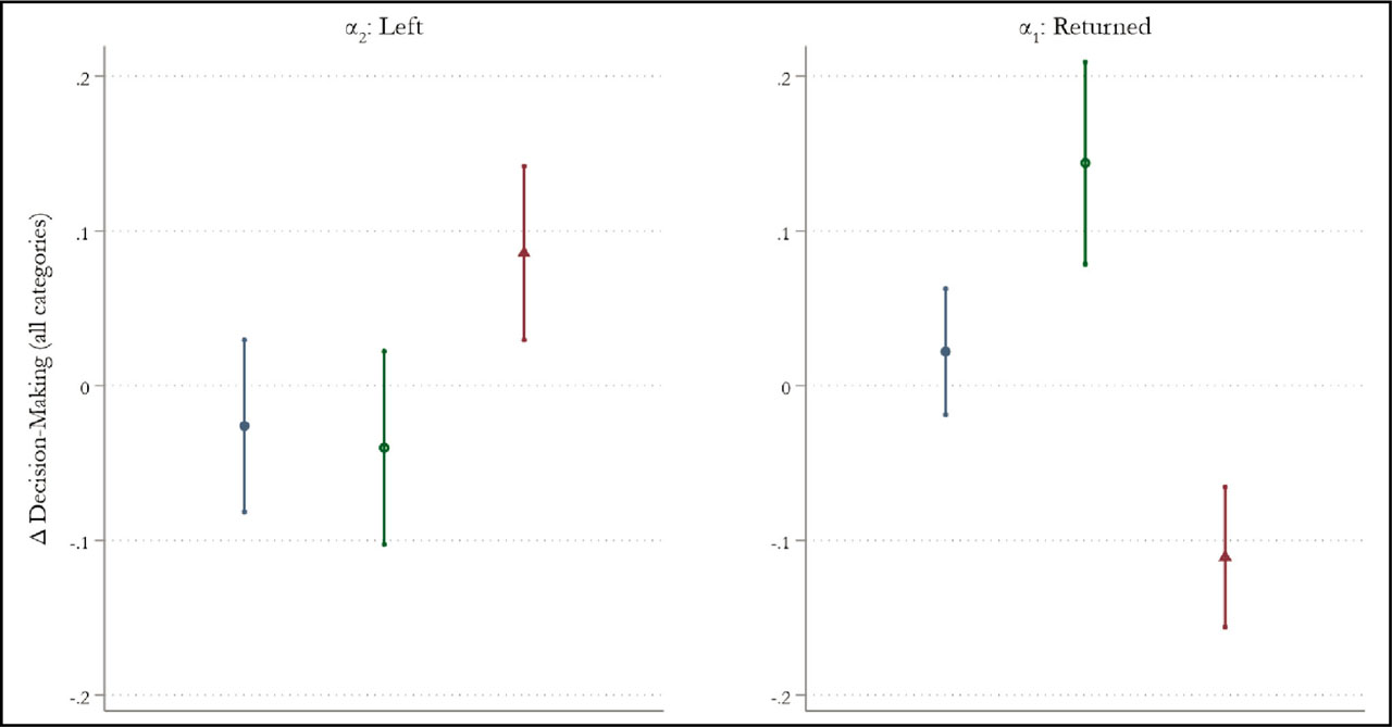
Figure 2
Persistence in women's decision-making power.
Fraction of Decisions Made by
•Husband Alone ○Husband+Wife ▴Wife Alone.
Coefficient plots of α2 (left panel) and α1 (right panel) from Eq. (4) are depicted (see Table F1 for coefficients listed in a table); 95% confidence intervals displayed, with robust standard errors clustered on VDC. The different colors/shapes each indicate a separate regression. Blue dots are from regressing husband's decision-making power on Eq. (4) and therefore represent changes in the fraction of decisions over which the husband has the only say. Hollow circles represent the change in the fraction of decisions made jointly. Hollow triangles represent the change in the wife's sole decision-making power. F-tests comparing the absolute value of α1 and α2 for the fraction of decisions made by the husband alone, the husband and wife jointly, and the wife alone yields p-values of 0.919, 0.036, and 0.557, respectively.
We find that when a husband leaves, the growth in decisions made by the wife alone is 9 percentage points differentially higher (or more positive) compared to changes over time periods when the husband's migration status does not change. At the same time, overall involvement (joint or alone) by the husband grows differentially lower (more negative or less positive), although these estimates are not statistically significant. However, if and when the husband returns, the wife forfeits all of the sole decision-making power she gained during the migration spell (11% lower growth rate). Yet, instead of being redistributed back to both the husband-only and joint decisions (as we might expect based on the changes when the husband leaves), decisions mostly shift to being made jointly. Specifically, there is a 14 percentage point greater growth in decisions made jointly upon the husband's return. An F-statistic comparing the absolute value of α1 to α2 (as reported in Table F1) for joint decisions has a p-value of 0.036, providing evidence that the growth in joint decisions upon the husband's return is larger than the low (or possibly negative) growth rate when he leaves. In other words, while the wife ultimately loses any sole decision-making power she had gained, there is suggestive evidence that, on net, she is left with more shared decision-making power than before her husband's migration spell. This is because the growth in joint decisions is differentially larger than the smaller (or perhaps negative) change in joint decisions estimated between the periods when the migrant leaves (coefficient is −0.040 but is statistically indistinguishable from zero).27
Even if women ultimately gain shared decision-making power after a husband returns, it may not ultimately affect the decisions the household makes. This could happen if, for instance, husbands have disproportionately more bargaining power and therefore household decisions are still more likely to reflect their preferences. Table 5 reports the results from the regression in Eq. (4) with changes in expenditures as the dependent variable. Each row represents a different regression with a different dependent variable.
Table 5
Dynamic shifts in expenditures: first-difference approach (asinh)
| α1: returned | α2: left | P-value: |α1| = |α2| | N | |
|---|---|---|---|---|
| Δ Temptation goods | 1.084*** (0.361) | −0.952** (0.386) | 0.819 | 3,491 |
| Δ Health care | 0.328 (0.369) | 0.672** (0.329) | 0.467 | 3,368 |
| Δ Ceremonies or celebrations | −0.403 (0.286) | −0.909*** (0.299) | 0.163 | 3,473 |
| Δ Child education | −0.310 (0.236) | −0.450* (0.258) | 0.615 | 3,389 |
| Δ Child clothing | −0.107 (0.213) | −0.119 (0.243) | 0.955 | 3,407 |
| Δ Adult women clothing | −0.027 (0.153) | −0.120 (0.165) | 0.693 | 3,563 |
Notes: Robust standard errors clustered at the VDC level are in parentheses. Each row represents a separate regression where Returned and Left represent dummies that describe the change in the husband's migrant status between the previous and current periods. The P-value is from an F-test testing for equality between the absolute values of the Returned coefficient and the Left coefficient. Controls for the base period are included. The control set across all regressions includes a separate dummy each for various shocks (the household experienced a natural disaster aside from the 2015 earthquake, serious illness, death of a household member, falling agricultural prices, decrease in income, or loss of employment), a Mercalli scale measure of earthquake intensity at the VDC level, a dummy indicating whether the husband has migration experience, a dummy indicating a resident mother-in-law, a dummy indicating a resident father-in-law, and a separate dummy each indicating when the control is missing. Zeros are imputed for missing values. All amounts are in rupees and transformed by the inverse hyperbolic sine.
Among the categories for which we observed a change in the main result – temptation goods, children's education, and children's clothing – there are no asymmetric changes. In fact, spending on temptation goods appears to rebound by almost the exact same amount. This underscores that even if migration may change who participates in decision-making, the relative bargaining position of the decision-makers may play a large role in what decisions are made. Nevertheless, any lasting changes in decision-making power are an important first step toward more-equitable decision-making.28
5. Habit Formation as a Mechanism
We have shown that when husbands migrate, decision-making power tends to shift toward the wife, and there is suggestive evidence that she retains some decision-making power after he returns. A natural next question is: what is driving this pattern?
When a household member migrates for work, the composition of the resident household members also changes, which could affect the household economic decision-making power through several channels. First, shifting control over household decisions to his wife could be purely practical, as the migrant is less able to manage the household from a distance. Second, a husband's migration could increase his wife's bargaining power: migration affects labor allocation not only by the migrant, but also by those at home (Abdulloev et al., 2014; Lokshin and Glinskaya, 2009), thus affecting each individual's relative contribution to household income.
In addition, geographic separation could introduce asymmetric information about household decisions, therefore allowing the wife to make de facto independent decisions about the household budget. Ashraf et al, (2015) present results from a field experiment in El Salvador, which show that migrants increase savings when they could easily monitor and control the savings account back home. Ambler (2015) uses another experiment in El Salvador to show that recipients send home more remittances when their income is revealed to their spouse. A third study by Chen (2013) in China shows that the decisions that change during migration spells were those not easily monitored from afar or after the husband's return.
If husbands and wives have heterogeneous preferences, any of these three channels would ultimately lead to different household decisions. We are unable to distinguish between these three channels in order to identify what exactly drives contemporaneous changes in decision-making. However, none of these explanations on their own are likely to explain the possibility of persistence over time. One potential explanation consistent with persistent effects is that the male migrant is “bringing home” norms and customs from their destinations. This seems unlikely since Nepali migrants mostly migrate to the Middle East, Far East, or to other cities within Nepal. These destinations are not known for their liberal gender norms, and if anything, we might expect this mechanism to result in fewer decisions being made by women upon the migrant's return.
In order to explain persistence, we suggest that a different mechanism must be at work: habit formation. According to Wood and Neal (2007), “Habits are learned dispositions to repeat past responses. They are triggered by features of the context that have covaried frequently with past performance, including performance locations, preceding actions in a sequence, and particular people.” In economics, the original model of habit formation by Becker and Murphy (1998) assumes that past consumption affects current utility (what Becker and Murphy describe as “rational addiction”). This assumption describes the inherent “stickiness” of habits. Once formed, habits are difficult to override.
Current habits may be triggered to form (or dissolve) when some sort of shock causes individuals to reevaluate their behavioral choices (Verplanken et al., 2008; Wood and Neal, 2009). For example, a move to a new city (Verplanken et al., 2008) or transferring to a new university (Wood et al., 2005) provides a sufficiently different context that encourages individuals to form new habits. Likewise, the migration of a prominent household decision-maker represents a similarly discontinuous change in context that disrupts the household's usual decision-making process.
Of course, new habits are not guaranteed to stick. When a male migrant returns, what is stopping the household from resorting to their previous decision-making habits? Becker and Murphy's original habit-formation model offers an explanation: current preferences evolve over time through a process of “learning by doing.”29 Put differently, current preferences are endogenous to past consumption patterns. Applied to our setting, this could mean one of the following: women learn how to make financial decisions; husbands learn that their wives can successfully handle the finances; or both. Through this learning process, both husbands and wives realize that the wife is capable of contributing to the decision-making process. The new habit sticks.
This learning process takes time. Therefore, we expect the habit to form more strongly in households with longer migration spells. We can test for this by estimating Eqs. (1)–(3) again, this time including an interaction for the situation that the trip was declared to last for >6 months. Table 6 reports the results of this approach using decisions aggregated across all categories as the outcome.30 The findings confirm that households with longer migration spells report more dramatic changes in decision-making. Women are more likely to have sole control over decisions when the husband is on a longer trip, and long-term migrant husbands are more likely to give up sole control over decisions. Importantly, this result is comparatively less consistent with the narrative that norms are being imported from the migrant's destination countries, which seems unlikely to work along the intensive margin. And, as noted earlier, the frequent destinations of these migration spells are not very consistent with the norms-import channel. Of course, interpreting these results as evidence for habit formation requires an assumption that households selecting into longer trips are not systematically different along dimensions that are correlated with changes in decision-making, above and beyond the included controls and FE.
Table 6
Heterogeneity by trip length: change in decision-making (all categories)
| (1) | (2) | (3) | (4) | |
|---|---|---|---|---|
| Dependent variable: husband alone | ||||
| Migrant | 0.00525 (0.0145) | 0.00860 (0.0152) | 0.00735 (0.0148) | 0.0209 (0.0257) |
| Migrant × ≥ 6 months | −0.0619*** (0.0144) | −0.0616*** (0.0152) | −0.0600*** (0.0152) | −0.0541** (0.0224) |
| N | 7,569 | 7,569 | 3,010 | 3,010 |
| Dep. variable: husband and wife jointly | ||||
| Migrant | −0.0784*** (0.0212) | −0.0975*** (0.0232) | −0.0905*** (0.0242) | −0.105*** (0.0356) |
| Migrant × ≥ 6 months | −0.0180 (0.0231) | −0.0184 (0.0224) | −0.0176 (0.0225) | −0.0274 (0.0362) |
| N | 7,569 | 7,569 | 3,010 | 3,010 |
| Dep. variable: wife alone | ||||
| Migrant | 0.0645*** (0.0178) | 0.0700*** (0.0194) | 0.0738*** (0.0210) | 0.0631* (0.0322) |
| Migrant × ≥ 6 months | 0.0478** (0.0221) | 0.0485** (0.0224) | 0.0467** (0.0224) | 0.0606* (0.0330) |
| N | 7,569 | 7,569 | 3,010 | 3,010 |
| Household FE | Yes | Yes | Yes | Yes |
| Controls | No | Yes | Yes | Yes |
| Limited sample | No | No | Yes | Yes |
| HH-specific time trends | No | No | No | Yes |
Notes: Robust standard errors clustered at the VDC level are in parentheses. Each column refers to different specifications, as noted. For each specification, we regress three different dependent variables: the fraction of decisions over which the husband solely, the husband and wife jointly, or the wife solely has control. For each regression, we report the coefficient on the dummy for the situation that a husband is currently migrating and the coefficient on this variable interacted with a dummy indicating that the migrant spell is at least 6 months long. As before, the control set across all regressions includes a separate dummy each for various shocks (the household experienced a natural disaster aside from the 2015 earthquake, serious illness, death of a household member, falling agricultural prices, decrease in income, or loss of employment), a Mercalli scale measure of earthquake intensity at the VDC level, a dummy indicating whether the husband has migration experience, a dummy indicating a resident mother-in-law, a dummy indicating a resident father-in-law, and a separate dummy each indicating when the control is missing. Zeros are imputed for missing values.
HH, household; VDC, Village Development Committees.
6. Conclusion
During a husband's migration spell, his wife may exert more control over household resources and therefore change how the household spends income. Given the prevalence of seasonal migration in developing countries, even these temporary changes could have consequences for economic development. The extent to which these changes persist after migration spells will magnify these consequences.
Using a panel data of rural Nepali households, we present evidence that a husband's migration leads to contemporaneous shifts in intrahousehold decision-making: a husband's absence increases the expenditure decisions over which the wife has full control by 10 percentage points. These households also shift away from expenditures on alcohol and tobacco in favor of children's education and clothing. We exploit the migration of sons – which increases household income but does not change decision-making – to show that this does not seem to be driven by an income effect.
To address the challenge of self-selection into migration and omitted variables that could threaten our interpretation of these findings, we rely on household FE, conditioning on eventual selection into migration, and including household-specific time trends. These approaches address the concern that time-invariant and time-variant unobservables among households, such as household risk aversion or differential income trajectories across households, drive our results. Our results provide a narrative largely consistent across these empirical strategies. We argue that this approach, in addition with the narrative that the results form as a whole, provides a compelling case for our interpretation.
One remaining challenge relates to the location of the consumer of the good. For each kind of expenditure, we do not directly observe the consumer. One might hypothesize that temptation goods are consumed more often by men than women. If this is the case, then when men migrate, expenditures on temptation goods will decline simply because the consumer is no longer present. This presents a challenge to the interpretation of our main results. Disentangling this channel presents an important area of future research. However, we believe that our results tell another story. First, shifts in decision-making power are strongest for temptation goods, but there is evidence for changes in other categories as well. These other categories include expenditures that are definitely not consumed by the male migrant (children's education and clothing; and adult women clothing). Our analysis of persistence is also relevant; women retain some decision-making power when male migrants return, which seems to reflect changes in decision-making that go beyond the absence of the primary consumer. This is true even in the temptation goods category.31 Finally, the discussion on habit formation provides a further clue that this is not the case. If the results are being driven by the absence of the consumer, then the length of the trip should not matter, yet Table 6 shows that longer migration spells induce more dramatic changes in decision-making.
One important contribution of our paper is to show that the economic decisions are more likely to be made jointly even after a male migrant returns. This could be driven by either the importation of norms from abroad or a habit-formation model. We find that migration spells that last longer have larger changes in decision-making, which we argue is relatively more consistent with a habit-formation model. This suggests that even temporary migration spells may help achieve gender equality in economic decision-making, with downstream effects on how households spend their income. When women play a role in decisions, they are more likely to invest in the next generation, increasing the likelihood that a pernicious cycle of intergenerational poverty can be broken.
The evidence presented in this paper suggests that a new habit of more-equitable household decision-making can be formed over a period of temporary migration. If the new habit “sticks” and women continue to take part in economic decisions, then it seems plausible that temporary male migration could provide a mechanism for lasting cultural change. Our analysis can only speak to short-term effects, but the results are promising. Women's labor force participation in Nepal, a key indicator of gender equality, offers suggestive evidence supporting this narrative. When compared to its South Asian neighbors, Nepali female labor force participation rate (LFPR) stands out: while nearly 80% of women participate in the labor force in Nepal, only 26% do in India.32 At the same time, Nepali men and women also report relatively progressive beliefs: among South Asian countries, Nepalis have the lowest rates of disagreement with the notion that it is okay for women to work (ILO, 2018). Could these relatively progressive beliefs and outcomes be due to Nepal's relatively high rates of male migrant work? More broadly, can migrant work, through accommodation of new habits, be a catalyst for changing gender norms? We leave these questions to future research.
Declarations
Competing interests
None.
Funding
Funding for this project was provided by the Feed the Future Innovation Lab for Assets and Market Access (AMA) at UC Davis (formerly BASIS), and the Bill and Melinda Gates Foundation (BMGF), and the United States Agency for International Development (USAID) as part of the Consultative Group for International Agricultural Research (CGIAR) Research Program on Agriculture for Nutrition and Health (A4NH) Gender and Assets in Agriculture Project Phase 2 (GAAP2) led by the International Food Policy Research Institute (IFPRI).
Acknowledgments
We thank Bolanle Atilola, Hiranya Baral, Neena Joshi, Nick Magnan, Dipesh Pokharel, Rajendra Pradhan, Samyam Shrestha, Ashika Sharma, Shruti Sharma, Sudhindra Sharma, Pranaya Sthapit, and William Thompson for logistical and research support. Diane Charlton, Nick Magnan, Ruth Meinzen-Dick, Kadeem Noray, Rohini Pande, Christiana Stoddard, and participants at the 2017 Agricultural & Applied Economics Association (AAEA) Annual Meeting and Evidence for Policy Design's Research Assistants Lab all provided helpful feedback. All errors are our own.
Appendices
Appendix
A. Appendix Figure/Tables
This section includes various appendix figures and tables referenced throughout the text.
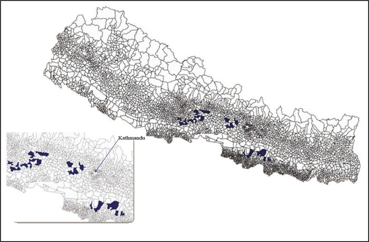
Figure A1
Village development committees representing seven districts in our data.
Note: The seven districts are Dhading, Mahotari, Nuwakot, Palpa, Rautahat, Sarlahi, and Tanahu.
Table A1
Changes in income and financial behavior (asinh) as the husband's migrant status changes
| (1) | (2) | (3) | (4) | |
|---|---|---|---|---|
| Annual income | 0.280** (0.130) | 0.173 (0.134) | 0.204 (0.135) | 0.004 (0.232) |
| N | 7,572 | 7,572 | 3,013 | 3,013 |
| Savings deposited in past month | 0.122 (0.085) | 0.092 (0.100) | 0.071 (0.112) | −0.173 (0.207) |
| N | 7,524 | 7,524 | 2,996 | 2,996 |
| Currently borrowing | 0.056 (0.217) | 0.269 (0.240) | 0.324 (0.269) | 0.139 (0.490) |
| N | 7,572 | 7,572 | 3,013 | 3,013 |
| Currently lending | −0.073 (0.184) | 0.016 (0.197) | −0.043 (0.224) | −0.299 (0.432) |
| N | 7,572 | 7,572 | 3,013 | 3,013 |
| Household and year FE | Yes | Yes | Yes | Yes |
| Controls | No | Yes | Yes | Yes |
| Limited sample | No | No | Yes | Yes |
| HH-specific time trends | No | No | No | Yes |
Notes: Robust standard errors clustered at the VDC level are in parentheses. Each coefficient displayed is from a separate regression and represents the coefficient on a binary variable indicating that the husband is currently migrating. All columns include household FE and year FE. The first column reports the results without any controls. The second and remaining columns include a control set: a separate dummy each for various shocks (the household experienced a natural disaster aside from the 2015 earthquake, serious illness, death of a household member, falling agricultural prices, decrease in income, or loss of employment), a Mercalli scale measure of earthquake intensity at the VDC level, a dummy indicating whether the husband has migration experience, a dummy indicating a resident mother-in-law, a dummy indicating a resident father-in-law, and a separate dummy each indicating when the control is missing. Zeros are imputed for missing values. Columns 3 and 4 are limited to the sample of households in which the husband migrates in any of the four rounds. Column 4 includes household-specific time trends. All amounts are in rupees and transformed by the inverse hyperbolic sine.
FE, fixed effects; HH, household; VDC, village development committee.
B. Migrant-son analysis
This section includes the tables corresponding to the migrant-son analysis.
Table B1
Shifts in decision-making power as son's migration status changes
| (1) | (2) | (3) | (4) | |
|---|---|---|---|---|
| Panel A: All categories | ||||
| Husband alone | −0.042*** (0.010) | −0.038*** (0.010) | −0.039*** (0.009) | −0.019 (0.016) |
| Husband and wife jointly | 0.010 (0.012) | 0.008 (0.012) | 0.010 (0.012) | 0.012 (0.021) |
| Wife alone | 0.011 (0.008) | 0.011 (0.008) | 0.012 (0.008) | 0.004 (0.015) |
| N | 7,569 | 7,569 | 4,025 | 4,025 |
| Panel B: Disaggregated by category | ||||
| Temptation goods | ||||
| Husband alone | 0.011 (0.011) | 0.008 (0.011) | 0.006 (0.011) | 0.029 (0.022) |
| Husband and wife jointly | 0.004 (0.011) | 0.005 (0.011) | 0.002 (0.011) | −0.008 (0.021) |
| Wife alone | 0.010 (0.007) | 0.010 (0.007) | 0.009 (0.008) | 0.004 (0.015) |
| N | 7,524 | 7,524 | 4,009 | 4,009 |
| Health care | ||||
| Husband alone | 0.001 (0.013) | 0.001 (0.013) | −0.004 (0.012) | −0.017 (0.018) |
| Husband and wife jointly | 0.023 (0.017) | 0.020 (0.017) | 0.023 (0.018) | 0.040 (0.031) |
| Wife alone | 0.012 (0.010) | 0.012 (0.010) | 0.014 (0.010) | 0 (0.017) |
| N | 7,564 | 7,564 | 4,020 | 4,020 |
| Ceremonies or celebrations | ||||
| Husband alone | 0.001 (0.012) | 0.001 (0.012) | −0.004 (0.012) | −0.007 (0.018) |
| Husband and wife jointly | 0.035** (0.016) | 0.031* (0.016) | 0.032* (0.017) | 0.044 (0.027) |
| Wife alone | 0.015 (0.013) | 0.015 (0.013) | 0.016 (0.013) | −0.002 (0.020) |
| N | 7,537 | 7,537 | 4,013 | 4,013 |
| Child education | ||||
| Husband alone | −0.003 (0.014) | −0.005 (0.014) | −0.009 (0.014) | −0.032 (0.019) |
| Husband and wife jointly | −0.043** (0.020) | −0.045** (0.020) | −0.035* (0.020) | −0.035 (0.035) |
| Wife alone | 0.010 (0.012) | 0.012 (0.013) | 0.016 (0.013) | 0.009 (0.023) |
| N | 7,415 | 7,415 | 3,897 | 3,897 |
| Child clothing | ||||
| Husband alone | 0.004 (0.013) | 0.002 (0.013) | −0.004 (0.012) | −0.023 (0.018) |
| Husband and wife jointly | −0.007 (0.020) | −0.009 (0.020) | 0.001 (0.020) | 0.007 (0.032) |
| Wife alone | 0.009 (0.013) | 0.012 (0.013) | 0.012 (0.013) | 0 (0.024) |
| N | 7,469 | 7,469 | 3,938 | 3,938 |
| Adult women clothing | ||||
| Husband alone | 0.008 (0.014) | 0.007 (0.014) | 0.001 (0.013) | −0.015 (0.020) |
| Husband and wife jointly | 0.013 (0.020) | 0.011 (0.020) | 0.011 (0.019) | −0.010 (0.038) |
| Wife alone | 0.008 (0.018) | 0.007 (0.018) | 0.012 (0.018) | 0.022 (0.025) |
| N | 7,553 | 7,553 | 4,013 | 4,013 |
| Household and year FE | Yes | Yes | Yes | Yes |
| Controls | No | Yes | Yes | Yes |
| Limited sample | No | No | Yes | Yes |
| HH-specific time trends | No | No | No | Yes |
Notes: Robust standard errors clustered at the VDC level are in parentheses. Each displayed coefficient is from a separate regression and represents the coefficient on a binary variable indicating that at least one son in the household is currently migrating. All columns include household FE and year FE. The first column reports the results without any controls. The second and remaining columns include a control set: a separate dummy each for various shocks (the household experienced a natural disaster aside from the 2015 earthquake, serious illness, death of a household member, falling agricultural prices, decrease in income, or loss of employment), a Mercalli scale measure of earthquake intensity at the VDC level, a dummy indicating whether the husband has migration experience, a dummy indicating a resident mother-in-law, a dummy indicating a resident father-in-law, and a separate dummy each indicating when the control is missing. Zeros are imputed for missing values. Columns 3 and 4 are limited to the sample of households wherein the husband migrates in any of the four rounds. Column 4 includes household-specific time trends. Outcome variables are fractions of decisions over which the decision-making power is distributed as described. Note that children's clothing includes expenditures on school uniforms. See Section C in the Appendix for more details on how these variables are composed.
FE, fixed effects; HH, household; VDC, village development committee.
Table B2
Shifts in expenditures (asinh) as son's migration status changes
| (1) | (2) | (3) | (4) | |
|---|---|---|---|---|
| Temptation goods | 0.176 (0.134) | 0.189 (0.129) | 0.134 (0.134) | 0.201 (0.243) |
| N | 7,417 | 7,417 | 3,956 | 3,956 |
| Health care | 0.221 (0.147) | 0.236 (0.149) | 0.199 (0.144) | 0.219 (0.275) |
| N | 7,145 | 7,145 | 3,811 | 3,811 |
| Ceremonies or celebrations | 0.122 (0.127) | 0.111 (0.129) | 0.111 (0.128) | 0.009 (0.221) |
| N | 7,407 | 7,407 | 3,939 | 3,939 |
| Child education | −0.351*** (0.128) | −0.357*** (0.128) | −0.262** (0.132) | −0.211 (0.177) |
| N | 7,339 | 7,339 | 3,845 | 3,845 |
| Child clothing | −0.089 (0.107) | −0.079 (0.106) | 0.006 (0.107) | −0.086 (0.160) |
| N | 7,349 | 7,349 | 3,839 | 3,839 |
| Adult women clothing | −0.059 (0.077) | −0.055 (0.076) | −0.045 (0.076) | −0.076 (0.136) |
| N | 7548 | 7548 | 4010 | 4010 |
| Household and year FE | Yes | Yes | Yes | Yes |
| Controls | No | Yes | Yes | Yes |
| Limited sample | No | No | Yes | Yes |
| HH-specific time trends | No | No | No | Yes |
Notes: Robust standard errors clustered at the VDC level are in parentheses. Each coefficient displayed is from a separate regression and represents the coefficient on a binary variable indicating that at least one son in the household is currently migrating. All columns include household FE and year FE. The first column reports the results without any controls. The second and remaining columns include a control set: a separate dummy each for various shocks (the household experienced a natural disaster aside from the 2015 earthquake, serious illness, death of a household member, falling agricultural prices, decrease in income, or loss of employment), a Mercalli scale measure of earthquake intensity at the VDC level, a dummy indicating whether the husband has migration experience, a dummy indicating a resident mother-in-law, a dummy indicating a resident father-in-law, and a separate dummy each indicating when the control is missing. Zeros are imputed for missing values. Columns 3 and 4 are limited to the sample of households in which the husband migrates in any of the four rounds. Column 4 includes household-specific time trends. All amounts are in rupees and transformed by the inverse hyperbolic sine.
FE, fixed effects; HH, household; VDC, village development committee.
Table B3
Changes in income and financial behavior (asinh) as son's migration status changes
| (1) | (2) | (3) | (4) | |
|---|---|---|---|---|
| Annual income | 0.497*** (0.156) | 0.524*** (0.163) | 0.541*** (0.164) | 0.509* (0.287) |
| N | 7,572 | 7,572 | 4,028 | 4,028 |
| Savings deposited in past month | 0.034 (0.082) | 0.027 (0.080) | 0.047 (0.080) | 0.110 (0.191) |
| N | 7,524 | 7,524 | 4,005 | 4,005 |
| Currently borrowing | 0.523*** (0.197) | 0.482** (0.196) | 0.496** (0.213) | 0.833** (0.405) |
| N | 7,572 | 7,572 | 4,028 | 4,028 |
| Currently lending | −0.117 (0.168) | −0.180 (0.167) | −0.164 (0.170) | 0.008 (0.275) |
| N | 7,572 | 7,572 | 4,028 | 4,028 |
| Household and year FE | Yes | Yes | Yes | Yes |
| Controls | No | Yes | Yes | Yes |
| Limited sample | No | No | Yes | Yes |
| HH-specific time trends | No | No | No | Yes |
Notes: Robust standard errors clustered at the VDC level are in parentheses. Each coefficient displayed is from a separate regression and represents the coefficient on a binary variable indicating that at least one son in the household is currently migrating. All columns include household FE and year FE. The first column reports the results without any controls. The second and remaining columns include a control set: a separate dummy each for various shocks (the household experienced a natural disaster aside from the 2015 earthquake, serious illness, death of a household member, falling agricultural prices, decrease in income, or loss of employment), a Mercalli scale measure of earthquake intensity at the VDC level, a dummy indicating whether the husband has migration experience, a dummy indicating a resident mother-in-law, a dummy indicating a resident father-in-law, and a separate dummy each indicating when the control is missing. Zeros are imputed for missing values. Columns 3 and 4 are limited to the sample of households in which the husband migrates in any of the four rounds. Column 4 includes household-specific time trends. All amounts are in rupees and transformed by the inverse hyperbolic sine.
FE, fixed effects; HH, household; VDC, village development committee.
Table B4
Characteristics by migrant status
| (1) | (2) | (3) | (4) | |
|---|---|---|---|---|
| Overall | Husband ever migrate | Son ever migrate | P-value (2) = (3) | |
| Panel A | ||||
| Husband characteristics | ||||
| Age | 46.119 | 38.934 | 51.839 | 0.000*** |
| [12.921] | [9.339] | [10.627] | ||
| Years of education | 5.104 | 6.219 | 4.553 | 0.000*** |
| [3.940] | [3.517] | [3.882] | ||
| Can read or write | 0.763 | 0.877 | 0.729 | 0.000*** |
| [0.365] | [0.270] | [0.377] | ||
| Wife characteristics | ||||
| Age | 41.650 | 35.076 | 47.247 | 0.000*** |
| [12.143] | [9.016] | [9.852] | ||
| Years of education | 2.513 | 3.770 | 1.584 | 0.000*** |
| [3.545] | [3.790] | [2.849] | ||
| Can read or write | 0.527 | 0.677 | 0.449 | 0.000*** |
| [0.401] | [0.369] | [0.378] | ||
| N | 2,508 | 979 | 1,317 | 1,923 |
| Panel B | ||||
| Household characteristics income (asinh) | 11.562 | 11.826 | 11.6073 | 0.000*** |
| [3.117] | [2.931] | [3.183] | ||
| No. of resident household members | 3.483 | 3.629 | 3.323 | 0.000*** |
| [1.854] | [1.745] | [1.877] | ||
| Resident mother-in-law | 0.230 | 0.316 | 0.158 | 0.000*** |
| [0.421] | [0.465] | [0.365] | ||
| Resident father-in-law | 0.159 | 0.232 | 0.088 | 0.000*** |
| [0.365] | [0.422] | [0.284] | ||
| Resident daughter-in-law | 0.185 | 0.084 | 0.308 | 0.000*** |
| [0.388] | [0.277] | [0.462] | ||
| Shocks | ||||
| Natural disaster (nonearthquake) | 0.044 | 0.039 | 0.052 | 0.011** |
| [0.206] | [0.194] | [0.222] | ||
| Serious illness | 0.223 | 0.213 | 0.223 | 0.214 |
| [0.416] | [0.409] | [0.417] | ||
| Death of household member | 0.055 | 0.053 | 0.054 | 0.959 |
| [0.228] | [0.225] | [0.226] | ||
| Falling agricultural prices | 0.131 | 0.109 | 0.128 | 0.000*** |
| [0.338] | [0.312] | [0.335] | ||
| Decrease in income | 0.155 | 0.134 | 0.154 | 0.003*** |
| [0.362] | [0.341] | [0.361] | ||
| Loss of employment | 0.023 | 0.020 | 0.023 | 0.251 |
| [0.151] | [0.141] | [0.150] | ||
| Mercalli scale 2015 earthquake | 6.926 | 6.870 | 6.922 | 0.006*** |
| [0.505] | [0.525] | [0.512] | ||
| N | 7,572 | 3,013 | 4,028 | 5,888 |
[i] Notes: This table reports mean values with standard deviations in brackets. Column 1 includes all households, Column 2 is limited to households in which the husband migrates at some point, and Column 3 is limited to households in which a son migrates at some point. Column 4 reports the p-value for a t-test of differences between columns 2 and 3. In Panel A, data are at the household level and characteristics are defined using the mean value over time (2014–2018) for each household. Data in Panel B are pooled 2014–2018 values. The averages of the nonearthquake shocks represent the fraction of households that experienced a given event (e.g., death of a household member) since the past round of data were collected.
C. Defining variables
In this section, we define our main outcome variables.
C1. Aggregating expenditure categories
The following paragraphs list the expenditure items that make up each category. For some categories, the expenditure items making up the category change between survey rounds. This is unlikely to affect our results in substantive ways because we include year (survey round) FE. Nevertheless, we document the changes here. These descriptions apply to both the decision-making variables and expenditure amount variables, unless otherwise stated. Although the questions covered over various recall periods, all expenditures are then transformed into monthly expenditures. If any one of the expenditure items within a category is missing, then the entire category is missing.
Temptation goods include all tobacco products (chewing tobacco, cigarettes, pipe smoking, and beedi) and products containing alcohol. For decision-making questions, respondents were asked this question within the context of a 1 month recall period. Expenditure amounts were asked over a recall period of 1 month for the first two rounds and over 1 week for the second two rounds.
Health care is intended to be comprehensive of all formal health care and omits traditional healing. The first two survey rounds ask the respondent to separately recall expenditures on medicines and medical supplies (3 months), consultation and treatment fees including gifts (3 months), laboratory and diagnostic fees (3 months), other medical expenses (3 months), and vaccinations/medical supplies/innoculations/doctor's fees (1 year). In the final two survey rounds, this was captured in a single question whereby the respondent was asked to recall all expenditures on medicine, doctor visits, dental visits, laboratory/test fees, hospital bed charges, diagnostic tests, ambulance contraceptives, and durable household medical equipment over the past 3 months.
Ceremonies and celebrations is a category intended to cover all costs associated with ceremonies (e.g., weddings) and celebrations (e.g., community festivals). The way this was covered between survey rounds varied greatly. Data from the first two rounds cover beads, jewelry, and other ceremonial items (1 year) and weddings, funerals, and festivals (1 year). The final two survey rounds asked for religious observances and festivals, weddings, funerals, and dowries, each for a recall period of 1 year.
Children's education includes school fees (e.g., registration and tuition) and school supplies (e.g., textbooks) for a recall period of 1 year. These expenditure items were asked separately in rounds 1–2 but combined for rounds 3–4. Note that this category omits school uniforms.
Children's clothing covers all clothing for children, including school uniforms, over the past year. These items were separated in the first two survey rounds but combined in the final two rounds.
Adult women's clothing includes any clothing for adult women.
C2. Choice set for composition of household decision-makers
The answers available to respondents for the decision-making question changed between the first two and last two rounds of data. For 2014 and 2016, respondents selected from the choices “I decide”, “the male head of the household decides”, “I decide jointly with the male head”, “I decide jointly with another member of the household”, “I decide jointly with someone outside the household”, “Not applicable”, and “Refused.” For 2016 and 2017, respondents simply listed up to three household members by name as the decision-makers. We make the assumption that in the first two rounds, “male head of household” refers to the husband, which allows us to harmonize our interpretation of survey responses over time. Note that the change in choices introduced new categories that were not possible earlier, e.g., a husband making a decision with somebody else in the household. Thus, in 2017–2018, we code “husband” and “husband and somebody else” as “husband alone”, the rationale being that in 2014 or 2016, “male head of household makes decision” would likely be the closest answer choice to the case where a husband decides with somebody else. Likewise, we code “husband and wife” and “husband, wife, and somebody else” as “husband and wife”.
Table C1
Decision-making outcomes by migrant status
| (1) | (2) | (3) | (4) | |
|---|---|---|---|---|
| Overall | Ever migrate | Never migrate | P-value (2) – (3) | |
| Panel A: All categories | ||||
| Husband alone | 0.136 | 0.105 | 0.156 | 0.000*** |
| [0.209] | [0.187] | [0.220] | ||
| Husband and wife jointly | 0.338 | 0.304 | 0.361 | 0.000*** |
| [0.313] | [0.313] | [0.310] | ||
| Wife alone | 0.108 | 0.177 | 0.062 | 0.000*** |
| [0.208] | [0.256] | [0.152] | ||
| Panel B: Disaggregated by category | ||||
| Temptation goods | ||||
| Husband alone | 0.192 | 0.157 | 0.214 | 0.000*** |
| [0.293] | [0.274] | [0.302] | ||
| Husband and wife jointly | 0.107 | 0.080 | 0.125 | 0.000*** |
| [0.254] | [0.224] | [0.270] | ||
| Wife alone | 0.042 | 0.044 | 0.040 | 0.268 |
| [0.146] | [0.151] | [0.143] | ||
| Health care | ||||
| Husband alone | 0.120 | 0.087 | 0.141 | 0.000*** |
| [0.274] | [0.234] | [0.296] | ||
| Husband and wife jointly | 0.418 | 0.364 | 0.454 | 0.000*** |
| [0.437] | [0.434] | [0.435] | ||
| Wife alone | 0.110 | 0.193 | 0.056 | 0.000*** |
| [0.277] | [0.348] | [0.199] | ||
| Ceremonies or celebrations | ||||
| Husband alone | 0.124 | 0.093 | 0.144 | 0.000*** |
| [0.288] | [0.252] | [0.308] | ||
| Husband and wife jointly | 0.479 | 0.432 | 0.510 | 0.000*** |
| [0.438] | [0.438] | [0.435] | ||
| Wife alone | 0.137 | 0.211 | 0.089 | 0.000*** |
| [0.300] | [0.359] | [0.241] | ||
| Child education | ||||
| Husband alone | 0.131 | 0.097 | 0.154 | 0.000*** |
| [0.325] | [0.283] | [0.348] | ||
| Husband and wife jointly | 0.387 | 0.391 | 0.384 | 0.528 |
| [0.474] | [0.475] | [0.474] | ||
| Wife alone | 0.128 | 0.245 | 0.049 | 0.000*** |
| [0.324] | [0.419] | [0.206] | ||
| Child clothing | ||||
| Husband alone | 0.124 | 0.096 | 0.144 | 0.000*** |
| [0.311] | [0.278] | [0.330] | ||
| Husband and wife jointly | 0.385 | 0.381 | 0.387 | 0.556 |
| [0.466] | [0.467] | [0.465] | ||
| Wife alone | 0.140 | 0.262 | 0.058 | 0.000*** |
| [0.331] | [0.424] | [0.216] | ||
| Adult women clothing | ||||
| Husband alone | 0.130 | 0.100 | 0.149 | 0.000*** |
| [0.336] | [0.301] | [0.356] | ||
| Husband and wife jointly | 0.459 | 0.382 | 0.510 | 0.000*** |
| [0.498] | [0.486] | [0.500] | ||
| Wife alone | 0.236 | 0.342 | 0.166 | 0.000*** |
| [0.424] | [0.474] | [0.372] | ||
| N | 7,572 | 3,013 | 4,559 | 7,572 |
[i] Notes: This table reports the mean values with standard deviations in brackets. Column 1 includes all households, Column 2 is limited to households in which the husband migrates at some point, and Column 3 is limited to households wherein the husband has not reported migrating during any survey round. Column 4 reports the p-value for a t-test of differences between columns 2 and 3. The data are at the household level and are pooled 2014–2018 values. Decision-making variables are fractions of decisions over which the decision-making power is distributed as described out of all categories included in the analysis: temptation goods, health care, ceremonies, children's education, children's clothing, and adult women's clothing. See the text of this section (Appendix Section C) for more details on how these variables are composed.
We acknowledge that these assumptions may not hold, especially because migrants are young and that the wife is more likely to live with the father-in-law or mother-in-law. The main concern is that the head of the household is not the husband, and rather it is the father-in-law. If the father-in-law is the migrant, then we would expect to observe no change in decision-making (or at least less change than if the woman's own husband migrated). This means that our estimates are likely biased downward, which is lessconcerning than if it worked in the opposite direction.
D. Sensitivity analysis related to definitions of variables
In this section, we test the sensitivity of our analysis to an alternative definition of “migrant” and consider alternative transformations of our expenditure variables.
In Section 2, we discussed how we define migration spells – based on residence – and how we cannot identify the reason why men are residing outside of the household in every round of data. However, the data include information on whether or not the residence is for a longer term (>6 months) and outside of Nepal. For the 3 years in which we do observe the purpose for residency outside the home, men are no more likely to be described as migrating for work based on length of the term or whether or not they live outside Nepal. Nevertheless, we perform the main analysis limiting our definition of a husband's migrant status to those who are residing outside the household for a longer term and outside of Nepal. The results are very similar – in many cases, estimates are larger in magnitude and more statistically significant. This confirms the relevancy of this research to the migration literature specifically, although we do not have a traditional measure of migration in these data (Appendix: Tables D1–D3).
We also consider alternative transformations of our expenditure variables. The results have minor sensitivity to how we specify the expenditure outcomes. Although the inverse hyperbolic sine is generally the best transformation to use when encountering many zeros, we test alternative ways of dealing with outliers in Tables D4–D6 of the Appendix: taking the log of x + 1, top-coding at the 95th percentile, and top-coding at the 99th percentile. The results for temptation goods remain robust in every case, but the results for children's education show sensitivity, especially in the top-coding specifications. Thus, we interpret our children's education result with more caution, although we are fairly confident that there is a positive change in children's education given that we see this in the log(x+1) specification, which is likely the second preferred way of specifying our result given how many zeros we observe.
Finally, we test whether the results are the same when we drop the final two rounds of data (Appendix: Table D7). As discussed in the text, this is to ensure that our results are not driven by the fact that men were asked to answer the expenditures module for the final two rounds of data. As in the main results, we see an increase in children's clothing/education expenditures and decrease in spending for temptation goods (albeit at a slightly lower magnitude). The change in children's education expenditures are no longer statistically significant in the specification without controls (Column 1), but this is not the preferred specification and therefore does not concern us.
Table D1
Changes in income and financial behavior (asinh) as the husband's migrant status changes – only considering migration spells outside of Nepal and lasting >6 months
| (1) | (2) | (3) | (4) | |
|---|---|---|---|---|
| Annual income | 0.361** (0.169) | 0.267 (0.165) | 0.245 (0.174) | 0.076 (0.226) |
| N | 7,572 | 7,572 | 2,197 | 2,197 |
| Savings deposited in past month | 0.245** (0.101) | 0.235** (0.109) | 0.332*** (0.120) | 0.062 (0.254) |
| N | 7,524 | 7,524 | 2,184 | 2,184 |
| Currently borrowing | −0.010 (0.271) | 0.152 (0.282) | 0.063 (0.310) | 0.022 (0.560) |
| N | 7,572 | 7,572 | 2,197 | 2,197 |
| Currently lending | 0.228 (0.214) | 0.362 (0.232) | 0.311 (0.258) | −0.026 (0.489) |
| N | 7,572 | 7,572 | 2,197 | 2,197 |
| Household and year FE | Yes | Yes | Yes | Yes |
| Controls | No | Yes | Yes | Yes |
| Limited sample | No | No | Yes | Yes |
| HH-specific time trends | No | No | No | Yes |
Notes: Robust standard errors clustered at the VDC level are in parentheses. Each coefficient displayed is from a separate regression and represents the coefficient on a binary variable indicating that the husband is currently migrating. All columns include household FE and year FE. The first column reports the results without any controls. The second and remaining columns include a control set: a separate dummy each for various shocks (the household experienced a natural disaster aside from the 2015 earthquake, serious illness, death of a household member, falling agricultural prices, decrease in income, or loss of employment), a Mercalli scale measure of earthquake intensity at the VDC level, a dummy indicating whether the husband has migration experience, a dummy indicating a resident mother-in-law, a dummy indicating a resident father-in-law, and a separate dummy each indicating when the control is missing. Zeros are imputed for missing values. Columns 3 and 4 are limited to the sample of households in which the husband migrates in any of the four rounds. Column 4 includes household-specific time trends. All amounts are in rupees and transformed by the inverse hyperbolic sine.
FE, fixed effects; HH, household; VDC, village development committee.
Table D2
Shifts in decision-making power as the husband's migrant status changes – only considering migration spells outside of Nepal and lasting >6 months
| (1) | (2) | (3) | (4) | |
|---|---|---|---|---|
| Panel A: all categories | ||||
| Husband alone | −0.059*** (0.011) | −0.055*** (0.010) | −0.056*** (0.010) | −0.050*** (0.014) |
| Husband and wife jointly | −0.095*** (0.017) | −0.105*** (0.018) | −0.105*** (0.019) | −0.103*** (0.032) |
| Wife alone | 0.115*** (0.014) | 0.116*** (0.016) | 0.121*** (0.016) | 0.121*** (0.025) |
| N | 7,569 | 7,569 | 2,194 | 2,194 |
| Panel B: disaggregated by category | ||||
| Temptation goods | ||||
| Husband alone | −0.102*** (0.013) | −0.101*** (0.014) | −0.105*** (0.014) | −0.107*** (0.024) |
| Husband and wife jointly | −0.031*** (0.010) | −0.041*** (0.012) | −0.039*** (0.013) | −0.034* (0.020) |
| Wife alone | 0.014** (0.006) | 0.014** (0.006) | 0.012* (0.007) | 0.005 (0.015) |
| N | 7,524 | 7,524 | 2,184 | 2,184 |
| Health care | ||||
| Husband alone | −0.037** (0.015) | −0.032** (0.015) | −0.032** (0.015) | −0.028 (0.020) |
| Husband and wife jointly | −0.152*** (0.023) | −0.171*** (0.021) | −0.167*** (0.023) | −0.163*** (0.048) |
| Wife alone | 0.158*** (0.021) | 0.168*** (0.021) | 0.170*** (0.023) | 0.169*** (0.037) |
| N | 7,564 | 7,564 | 2,194 | 2,194 |
| Ceremonies or celebrations | ||||
| Husband alone | −0.049*** (0.016) | −0.044*** (0.016) | −0.046*** (0.016) | −0.033 (0.021) |
| Husband and wife jointly | −0.095*** (0.023) | −0.103*** (0.024) | −0.106*** (0.025) | −0.100** (0.047) |
| Wife alone | 0.130*** (0.019) | 0.132*** (0.021) | 0.140*** (0.023) | 0.130*** (0.039) |
| N | 7,537 | 7,537 | 2,184 | 2,184 |
| Child education | ||||
| Husband alone | −0.063*** (0.019) | −0.056*** (0.017) | −0.049*** (0.016) | −0.036 (0.022) |
| Husband and wife jointly | −0.087*** (0.027) | −0.088*** (0.027) | −0.094*** (0.029) | −0.108** (0.048) |
| Wife alone | 0.161*** (0.023) | 0.160*** (0.025) | 0.170*** (0.027) | 0.181*** (0.037) |
| N | 7,415 | 7,415 | 2,171 | 2,171 |
| Child clothing | ||||
| Husband alone | −0.071*** (0.018) | −0.067*** (0.017) | −0.063*** (0.017) | −0.053** (0.023) |
| Husband and wife jointly | −0.121*** (0.029) | −0.123*** (0.030) | −0.127*** (0.031) | −0.152*** (0.048) |
| Wife alone | 0.186*** (0.025) | 0.186*** (0.028) | 0.194*** (0.030) | 0.206*** (0.045) |
| N | 7,469 | 7,469 | 2,182 | 2,182 |
| Adult women clothing | ||||
| Husband alone | −0.049** (0.020) | −0.040** (0.019) | −0.042** (0.020) | −0.035 (0.024) |
| Husband and wife jointly | −0.162*** (0.023) | −0.180*** (0.022) | −0.175*** (0.024) | −0.190*** (0.047) |
| Wife alone | 0.170*** (0.018) | 0.179*** (0.020) | 0.185*** (0.020) | 0.196*** (0.045) |
| N | 7,553 | 7,553 | 2,192 | 2,192 |
| Household and year FE | Yes | Yes | Yes | Yes |
| Controls | No | Yes | Yes | Yes |
| Limited sample | No | No | Yes | Yes |
| HH-specific time trends | No | No | No | Yes |
Notes: Robust standard errors clustered at the VDC level are in parentheses. Each coefficient displayed is from a separate regression and represents the coefficient on a binary variable indicating that the husband is currently migrating. All columns include household FE and year FE. The first column reports the results without any controls. The second and remaining columns include a control set: a separate dummy each for various shocks (the household experienced a natural disaster aside from the 2015 earthquake, serious illness, death of a household member, falling agricultural prices, decrease in income, or loss of employment), a Mercalli scale measure of earthquake intensity at the VDC level, a dummy indicating whether the husband has migration experience, a dummy indicating a resident mother-in-law, a dummy indicating a resident father-in-law, and a separate dummy each indicating when the control is missing. Zeros are imputed for missing values. Columns 3 and 4 are limited to the sample of households wherein the husband migrates in any of the four rounds. Column 4 includes household-specific time trends. Outcome variables are fractions of decisions over which the decision-making power is distributed as described. Note that children's clothing includes expenditures on school uniforms. See Section C of the Appendix for more details on how these variables are composed.
FE, fixed effects; HH, household; VDC, village development committee.
Table D3
Shifts in expenditures (asinh) as the husband's migrant status changes – only considering migration spells outside of Nepal and lasting >6 months
| (1) | (2) | (3) | (4) | |
|---|---|---|---|---|
| Temptation goods | −1.325*** (0.180) | −1.427*** (0.179) | −1.482*** (0.170) | −1.589*** (0.328) |
| N | 7,417 | 7,417 | 2,144 | 2,144 |
| Health care | −0.051 (0.194) | −0.089 (0.217) | −0.090 (0.229) | 0.035 (0.354) |
| N | 7,145 | 7,145 | 2,083 | 2,083 |
| Ceremonies or celebrations | 0.135 (0.111) | 0.124 (0.114) | 0.137 (0.109) | −0.179 (0.225) |
| N | 7,407 | 7,407 | 2,155 | 2,155 |
| Child education | 0.226** (0.112) | 0.312*** (0.114) | 0.285** (0.111) | −0.078 (0.182) |
| N | 7,339 | 7,339 | 2,155 | 2,155 |
| Child clothing | 0.338*** (0.108) | 0.360*** (0.109) | 0.320*** (0.107) | 0.204 (0.175) |
| N | 7,349 | 7,349 | 2,161 | 2,161 |
| Adult women clothing | 0.043 (0.073) | 0.069 (0.077) | 0.064 (0.082) | 0.165 (0.148) |
| N | 7,548 | 7,548 | 2,191 | 2,191 |
| Household and year FE | Yes | Yes | Yes | Yes |
| Controls | No | Yes | Yes | Yes |
| Limited sample | No | No | Yes | Yes |
| HH-specific time trends | No | No | No | Yes |
Notes: Robust standard errors clustered at the VDC level are in parentheses. Each coefficient displayed is from a separate regression and represents the coefficient on a binary variable indicating that the husband is currently migrating. All columns include household FE and year FE. The first column reports the results without any controls. The second and remaining columns include a control set: a separate dummy each for various shocks (the household experienced a natural disaster aside from the 2015 earthquake, serious illness, death of a household member, falling agricultural prices, decrease in income, or loss of employment), a Mercalli scale measure of earthquake intensity at the VDC level, a dummy indicating whether the husband has migration experience, a dummy indicating a resident mother-in-law, a dummy indicating a resident father-in-law, and a separate dummy each indicating when the control is missing. Zeros are imputed for missing values. Columns 3 and 4 are limited to the sample of households in which the husband migrates in any of the four rounds. Column 4 includes household-specific time trends. All amounts are in rupees and transformed by the inverse hyperbolic sine.
FE, fixed effects; HH, household; VDC, village development committee.
Table D4
Changes in expenditures, income, and financial behavior as the husband's migrant status changes – log(x+1)
| (1) | (2) | (3) | (4) | |
|---|---|---|---|---|
| Panel A: expenditures | ||||
| Temptation goods | −0.951*** (0.153) | −1.086*** (0.161) | −1.066*** (0.159) | −1.072*** (0.280) |
| N | 7,417 | 7,417 | 2,940 | 2,940 |
| Health care | −0.013 (0.131) | −0.035 (0.152) | −0.032 (0.158) | 0.233 (0.275) |
| N | 7,145 | 7,145 | 2,850 | 2,850 |
| Ceremonies or celebrations | 0.035 (0.097) | 0.006 (0.092) | 0.056 (0.102) | −0.187 (0.220) |
| N | 7,407 | 7,407 | 2,948 | 2,948 |
| Children's education | 0.154* (0.092) | 0.246** (0.096) | 0.163* (0.099) | −0.176 (0.162) |
| N | 7,339 | 7,339 | 2,954 | 2,954 |
| Children's clothing | 0.351*** (0.088) | 0.401*** (0.094) | 0.399*** (0.098) | 0.163 (0.151) |
| N | 7,349 | 7,349 | 2,965 | 2,965 |
| Adult women's clothing | −0.062 (0.058) | −0.049 (0.059) | −0.022 (0.059) | 0.022 (0.115) |
| N | 7,548 | 7,548 | 3,005 | 3,005 |
| Panel B: income and financial behavior | ||||
| Annual income | 0.281** (0.124) | 0.177 (0.128) | 0.208 (0.129) | 0.023 (0.221) |
| N | 7,572 | 7,572 | 3,013 | 3,013 |
| Savings deposited in past month | 0.109 (0.076) | 0.085 (0.090) | 0.064 (0.102) | −0.155 (0.189) |
| N | 7,524 | 7,524 | 2,996 | 2,996 |
| Currently borrowing | 0.055 (0.204) | 0.254 (0.225) | 0.304 (0.253) | 0.131 (0.461) |
| N | 7,572 | 7,572 | 3,013 | 3,013 |
| Currently lending | −0.068 (0.173) | 0.016 (0.185) | −0.040 (0.210) | −0.282 (0.406) |
| N | 7,572 | 7,572 | 3,013 | 3,013 |
| Household and year FE | Yes | Yes | Yes | Yes |
| Controls | No | Yes | Yes | Yes |
| Limited sample | No | No | Yes | Yes |
| HH-specific time trends | No | No | No | Yes |
Notes: Robust standard errors clustered at the VDC level are in parentheses. Each coefficient displayed is from a separate regression and represents the coefficient on a binary variable indicating that the husband is currently migrating. All columns include household FE and year FE. The first column reports the results without any controls. The second and remaining columns include a control set: a separate dummy each for various shocks (the household experienced a natural disaster aside from the 2015 earthquake, serious illness, death of a household member, falling agricultural prices, decrease in income, or loss of employment), a Mercalli scale measure of earthquake intensity at the VDC level, a dummy indicating whether the husband has migration experience, a dummy indicating a resident mother-in-law, a dummy indicating a resident father-in-law, and a separate dummy each indicating when the control is missing. Zeros are imputed for missing values. Columns 3 and 4 are limited to the sample of households in which the husband migrates in any of the four rounds. Column 4 includes household-specific time trends.
FE, fixed effects; HH, household; VDC, village development committee.
Table D5
Changes in expenditures, income, and financial behavior as the husband's migrant status changes – top-coded at the 99th percentile
| (1) | (2) | (3) | (4) | |
|---|---|---|---|---|
| Panel A: expenditures | ||||
| Temptation goods | −120.197** (53.600) | −123.775** (53.349) | −103.070* (58.289) | −84.433 (89.528) |
| N | 7,417 | 7,417 | 2,940 | 2,940 |
| Health care | −142.523 (209.494) | 67.791 (208.082) | 37.156 (213.112) | 384.495 (441.580) |
| N | 7,145 | 7,145 | 2,850 | 2,850 |
| Ceremonies or celebrations | −61.221 (200.328) | −98.690 (207.853) | −101.441 (244.901) | −69.571 (428.462) |
| N | 7,407 | 7,407 | 2,948 | 2,948 |
| Children's education | 46.994 (70.327) | 57.460 (80.099) | 32.590 (86.554) | −17.220 (91.988) |
| N | 7,339 | 7,339 | 2,954 | 2,954 |
| Children's clothing | 66.530*** (19.940) | 66.780*** (19.517) | 68.799*** (21.046) | 43.934 (46.406) |
| N | 7,349 | 7,349 | 2,965 | 2,965 |
| Adult women's clothing | −12.056 (17.752) | −11.160 (18.640) | −5.324 (18.132) | 22.142 (36.732) |
| N | 7,548 | 7,548 | 3,005 | 3,005 |
| Panel B: income and financial behavior | ||||
| Annual income | 47,989.637*** (10,443.880) | 42,926.326*** (10,572.657) | 40,291.132*** (12,732.178) | 46,886.496** (20,457.034) |
| N | 7,572 | 7,572 | 3,013 | 3,013 |
| Savings deposited in past month | 26.565 (117.086) | 65.817 (133.244) | 33.088 (151.638) | 63.081 (288.894) |
| N | 7,524 | 7,524 | 2,996 | 2,996 |
| Currently borrowing | −4,592.633 (5,078.635) | −4,186.492 (5,943.972) | −7,271.935 (6,512.158) | −4,250.191 (11,469.621) |
| N | 7,572 | 7,572 | 3,013 | 3,013 |
| Currently lending | −499.550 (1,535.515) | 538.604 (1,651.946) | 154.814 (1,959.374) | −2,634.804 (3,550.470) |
| N | 7,572 | 7,572 | 3,013 | 3,013 |
| Household and year FE | Yes | Yes | Yes | Yes |
| Controls | No | Yes | Yes | Yes |
| Limited sample | No | No | Yes | Yes |
| HH-specific time trends | No | No | No | Yes |
Notes: Robust standard errors clustered at the VDC level are in parentheses. Each coefficient displayed is from a separate regression and represents the coefficient on a binary variable indicating that the husband is currently migrating. All columns include household FE and year FE. The first column reports the results without any controls. The second and remaining columns include a control set: a separate dummy each for various shocks (the household experienced a natural disaster aside from the 2015 earthquake, serious illness, death of a household member, falling agricultural prices, decrease in income, or loss of employment), a Mercalli scale measure of earthquake intensity at the VDC level, a dummy indicating whether the husband has migration experience, a dummy indicating a resident mother-in-law, a dummy indicating a resident father-in-law, and a separate dummy each indicating when the control is missing. Zeros are imputed for missing values. Columns 3 and 4 are limited to the sample of households in which the husband migrates in any of the four rounds. Column 4 includes household-specific time trends.
FE, fixed effects; HH, household; VDC, village development committee.
Table D6
Changes in expenditures, income, and financial behavior as the husband's migrant status changes – top-coded at the 95th percentile
| (1) | (2) | (3) | (4) | |
|---|---|---|---|---|
| Panel A: expenditures | ||||
| Temptation goods | −126.360*** (38.072) | −137.050*** (38.904) | −117.563*** (39.783) | −103.698 (63.795) |
| N | 7,417 | 7,417 | 2,940 | 2,940 |
| Health care | −75.066 (133.753) | −3.897 (121.987) | −36.762 (119.550) | 154.302 (255.985) |
| N | 7,145 | 7,145 | 2,850 | 2,850 |
| Ceremonies or celebrations | −91.457 (92.147) | −121.699 (94.857) | −98.522 (116.511) | −163.506 (172.497) |
| N | 7,407 | 7,407 | 2,948 | 2,948 |
| Children's education | 47.410 (37.658) | 58.955 (41.153) | 29.104 (44.499) | −70.578 (63.297) |
| N | 7,339 | 7,339 | 2,954 | 2,954 |
| Children's clothing | 47.525*** (16.438) | 46.156*** (16.379) | 48.749*** (17.297) | 22.596 (34.274) |
| N | 7,349 | 7,349 | 2,965 | 2,965 |
| Adult women's clothing | −7.454 (13.565) | −3.645 (14.699) | 1.919 (14.565) | 13.527 (27.480) |
| N | 7,548 | 7,548 | 3,005 | 3,005 |
| Panel B: income and financial behavior | ||||
| Annual income | 42,899.597*** (7,854.542) | 40,695.726*** (8,243.078) | 39,730.933*** (10,362.565) | 48,730.244***(15,369.961) |
| N | 7,572 | 7,572 | 3,013 | 3,013 |
| Savings deposited in past month | 11.375 (23.572) | 18.660 (28.278) | 10.282 (33.734) | −5.363 (56.177) |
| N | 7,524 | 7,524 | 2,996 | 2,996 |
| Currently borrowing | 1,178.234 (3,369.408) | 2,149.937 (3,874.228) | 201.140 (4,213.134) | −2,007.624 (8,311.890) |
| N | 7,572 | 7,572 | 3,013 | 3,013 |
| Currently lending | 53.964 (667.219) | 536.425 (749.997) | 120.092 (909.763) | −1,694.717 (1,763.982) |
| N | 7,572 | 7,572 | 3,013 | 3,013 |
| Household and year FE | Yes | Yes | Yes | Yes |
| Controls | No | Yes | Yes | Yes |
| Limited sample | No | No | Yes | Yes |
| HH-specific time trends | No | No | No | Yes |
Notes: Robust standard errors clustered at the VDC level are in parentheses. Each coefficient displayed is from a separate regression and represents the coefficient on a binary variable indicating that the husband is currently migrating. All columns include household FE and year FE. The first column reports the results without any controls. The second and remaining columns include a control set: a separate dummy each for various shocks (the household experienced a natural disaster aside from the 2015 earthquake, serious illness, death of a household member, falling agricultural prices, decrease in income, or loss of employment), a Mercalli scale measure of earthquake intensity at the VDC level, a dummy indicating whether the husband has migration experience, a dummy indicating a resident mother-in-law, a dummy indicating a resident father-in-law, and a separate dummy each indicating when the control is missing. Zeros are imputed for missing values. Columns 3 and 4 are limited to the sample of households in which the husband migrates in any of the four rounds. Column 4 includes household-specific time trends.
FE, fixed effects; HH, household; VDC, village development committee.
Table D7
Shifts in expenditures (asinh) as the husband's migrant status changes – only considering the first two rounds of data
| (1) | (2) | (3) | |
|---|---|---|---|
| Temptation goods | −0.921*** (0.228) | −1.154*** (0.232) | −1.400*** (0.319) |
| N | 4,352 | 4,352 | 1,540 |
| Health care | 0.052 (0.189) | 0.029 (0.224) | −0.012 (0.371) |
| N | 4,016 | 4,016 | 1,426 |
| Ceremonies or celebrations | 0.113 (0.135) | −0.134 (0.137) | −0.086 (0.222) |
| N | 4,338 | 4,338 | 1,554 |
| Child education | 0.149 (0.155) | 0.415** (0.180) | 0.543** (0.242) |
| N | 4,270 | 4,270 | 1,558 |
| Child clothing | 0.289** (0.140) | 0.423*** (0.161) | 0.456** (0.209) |
| N | 4,286 | 4,286 | 1,572 |
| Adult women clothing | −0.053 (0.098) | 0.071 (0.107) | 0.160 (0.186) |
| N | 4,530 | 4,530 | 1,618 |
| Household and year FE | Yes | Yes | Yes |
| Controls | No | Yes | Yes |
| Limited sample | No | No | Yes |
| HH-specific time trends | No | No | No |
Notes: Robust standard errors clustered at the VDC level are in parentheses. Each coefficient displayed is from a separate regression and represents the coefficient on a binary variable indicating that the husband is currently migrating. All columns include household FE and year FE. The first column reports the results without any controls. The second and remaining columns include a control set: a separate dummy each for various shocks (the household experienced a natural disaster aside from the 2015 earthquake, serious illness, death of a household member, falling agricultural prices, decrease in income, or loss of employment), a Mercalli scale measure of earthquake intensity at the VDC level, a dummy indicating whether the husband has migration experience, a dummy indicating a resident mother-in-law, a dummy indicating a resident father-in-law, and a separate dummy each indicating when the control is missing. Zeros are imputed for missing values. Columns 3 and 4 are limited to the sample of households in which the husband migrates in any of the four rounds. All amounts are in rupees and transformed by the inverse hyperbolic sine.
FE, fixed effects; HH, household; VDC, village development committee.
E. Attrition analysis
Our main data source is an unbalanced panel of rural Nepali households residing in 60 village development committees (VDCs).33 Within each VDC, the original sample was stratified based on geography, with 25 households selected from a central tole (neighborhood) in the centermost ward, 15 households selected from a noncentral tole in the centermost ward, 10 households from a ward adjacent to the centermost ward, and 10 households from a nonadjacent ward.
Moreover, 43% of the households in our sample are interviewed all four rounds, while the remaining are interviewed for only two (41%) or three (15%) rounds. Households drop out of the sample (attrition) as a result of either inability to locate respondents,34 a common issue in this context (“not found”), or (b) the purposeful removal of some households from the sample (“dropped”). The latter occurred after the 2015 earthquake disrupted the rollout of the intervention for which the data were being collected. In response to this change, all households living in 10 VDCs within two districts, Nuwakot and Dhading, were not interviewed again in 2017 or 2018. In the remaining districts, all households living in noncentral wards were also removed from the sample. Table E1 describes how the sample size changes over time.
A first-order concern is that migration is related to attrition, therefore causing our treatment and counterfactual groups to have different rates of attrition. Presumably, attrition is related to certain factors — e.g., in the case of purposeful attrition, two entire districts were dropped because of greater exposure to the earthquake. Thus, differential rates of attrition would lead to treatment and counterfactual groups being less comparable.35 Table E2 also shows that attrition is not likely to be related to migration, conditional on the same set of controls, FE, and time trends as in the main specification. There is some evidence that migration of the husband predicts future absence among the limited sample (Column 3), which underscores why we show multiple specifications throughout the paper.36 In the first row, we consider attrition for any reason. In the next rows, we consider attrition due to being unable to locate the respondent and attrition due to households being purposely dropped from the sample. The latter only occurs in 2017, so we cannot include household-specific time trends. We can see that there is no relationship between any type of attrition and a husband's migration.
Nevertheless, despite similar rates of attrition between treatment and counterfactual groups over time, we might be concerned that the types of people who leave the sample in the treatment group are systematically different from those who leave the counterfactual group. Again, this would lead to the treatment group being less comparable to the counterfactual group. To evaluate this concern, we regress descriptive characteristics on dummies for both types of attrition, the husband's migration, and the interaction between migration and attrition (Table E3)37:
Table E1
Attrition over time
| (1) | (2) | (3) | (4) | |
|---|---|---|---|---|
| 2014 | 2016 | 2017 | 2018 | |
| Full sample | 2,508 | 2,281 | 1,456 | 1,327 |
| Attrition (not found) | . | 227 | 165 | 294 |
| Attrition (dropped) | . | 0 | 887 | 887 |
[i] Notes: The table reports the number of women in each category. Women leave the sample because either the surveyors could not locate the household/respondent or the households were purposely dropped (due to either the earthquake or other reasons necessary for the randomized evaluation's study design). Attrition numbers are cumulative (the columns will always add up to the full sample in 2014). See Section E in the Appendix for more details.
Table E2
Husband's migration and household attrition
| (1) | (2) | (3) | (4) | |
|---|---|---|---|---|
| Absent in next round | −0.020 (0.019) | 0.002 (0.022) | 0.046** (0.022) | −0.042 (0.038) |
| N | 6,225 | 6,225 | 2,465 | 2,465 |
| Not found | −0.002 (0.015) | 0.019 (0.017) | 0.024 (0.018) | −0.042 (0.038) |
| N | 6,225 | 6,225 | 2,465 | 2,465 |
| Dropped | −0.017 (0.016) | −0.017 (0.016) | 0.022 (0.015) | - |
| N | 6,225 | 6,225 | 2,465 | - |
| Household and year FE | Yes | Yes | Yes | Yes |
| Controls | No | Yes | Yes | Yes |
| Limited sample | No | No | Yes | Yes |
| HH-specific time trends | No | No | No | Yes |
Notes: Robust standard errors clustered at the VDC level are in parentheses. Each coefficient displayed is from a separate regression and represents the coefficient on a binary variable indicating that the husband is currently migrating. The control set across all regressions includes a separate dummy each for the situation that the household experienced a natural disaster (aside from the 2015 earthquake), serious illness, death of a household member, falling agricultural prices, decrease in income, or loss of employment, a Mercalli scale measure of earthquake intensity at the VDC level, and a separate dummy each indicating when the control is missing. Zeros are imputed for missing values. Even columns limit the sample to households in which the husband migrates in any of the four rounds. The last two columns include household-specific time trends, in addition to the control set. Absent in next round – dropped is not estimated in the final two columns because the outcome is perfectly collinear with household-specific time trends. See Section E of the Appendix for more detail.
FE, fixed effects; HH, household; VDC, village development committee.
Table E3
Selection into attrition by migration status over time
| (1) | (2) | (3) | (4) | (5) | (6) | |
|---|---|---|---|---|---|---|
| Not found | Dropped | Current migrant | Not found × current migrant | Dropped × current migrant | N | |
| Household characteristics | ||||||
| No. of resident household members | 0.042 | 0.098 | 0.270*** | 0.103 | −0.152 | 6,245 |
| Resident mother-in-law | 0.020 | −0.019 | 0.144*** | 0.121*** | 0.020 | 6,245 |
| Resident father-in-law | 0.009 | −0.010 | 0.113*** | 0.089** | 0.049 | 6,245 |
| Resident daughter-in-law | 0.040* | −0.015 | −0.165*** | −0.041 | 0.012 | 6,245 |
| Household shocks | ||||||
| Natural disaster (nonearthquake) | −0.002 | 0.028** | −0.008 | 0.005 | −0.004 | 6,227 |
| Serious illness | 0.039* | 0.023 | −0.029** | −0.083* | 0.061 | 6,231 |
| Death of household member | 0.018 | 0.019* | −0.016** | 0.026 | 0.017 | 6,229 |
| Falling agricultural prices | −0.007 | 0.205*** | −0.021* | −0.049** | −0.046 | 6,116 |
| Decrease in income | −0.016 | 0.243*** | −0.039*** | −0.032 | −0.045 | 6,130 |
| Loss of employment | 0.014 | 0.013* | −0.014*** | −0.006 | −0.013 | 6,217 |
| Mercalli scale 2015 earthquake | −0.264 | 5.278*** | −0.229** | 0.710** | 0.037 | 6,245 |
Notes: Each row represents a different regression in which the outcome variable is either a household characteristic or shock. Robust standard errors clustered at the VDC level are in parentheses. Column 1 lists the coefficient on a dummy for the situation that the respondent was absent in the next period because they could not be located. Column 2 lists the coefficient on the dummy if the respondent was absent in the next round because they were dropped from the sample on purpose. Column 3 lists the coefficient on a variable indicating that the husband is migrating during the current time period. The fourth and fifth columns show the interactions between the previous columns. The sixth column lists the sample size for each regression.
VDC, village development committee.
In the equation above, Yit−1 and CurrentMigrantit−1 represent descriptive characteristics and a dummy for the husband's migration in the previous period. Therefore, the coefficients listed in columns 4 and 5 of Table E3 represent the change in a given characteristic between the treatment group and counterfactual group within the attrition sample (either “not found” or purposely “dropped”). Among households that were purposely dropped, there are no observable differences between the migrants and the nonmigrants. However, among households that were not located in the next period, those with a husband migrating were more likely to reside with parents-in-law, less likely to experience a serious illness or falling agriculture prices, and had more exposure to the earthquake by 0.710 Mercalli scale points. We can (and do) directly control for economic shocks, so this is only a concern if shocks are correlated with unobservables varying in a nonlinear manner over time at the household level.
In our main regression, we condition on observables, household FE, and in some cases, household-specific time trends. Therefore, characteristics that are different would have to vary above and beyond these things (e.g., a type of economic shock not captured in the survey). Nevertheless, this exercise gives us a sense of whether unobservables of this nature are likely to be a concern.
F. Exploring persistence
F.1. Persistence in women's decision-making power
Table F1 reports the results of Eq. (4) with the decision-making outcomes as the dependent variable. Each row represents a different regression, where the coefficients Returnedit and Leftit are reported in each column. Column 3 reports a p-value for the F-test |α1| = |α2|. The results in Panel A correspond directly to Figure 2.
F2. Alternative specifications
Table F2 reports the results of Eq. (4) while also including an indicator for whether the husband is migrating in both t and t – 1. The omitted group are households for whom the husband is home in both periods.
Table F1
Dynamic shifts in decision-making power between husband and wife: first-difference approach
| α1: returned | α2: left | P-value: |α1| = |α2| | N | |
|---|---|---|---|---|
| Panel A: Δ All categories | ||||
| Husband alone | 0.022 (0.020) | −0.026 (0.028) | 0.919 | 3,580 |
| Husband and wife jointly | 0.144*** (0.032) | −0.040 (0.031) | 0.036** | 3,580 |
| Wife alone | −0.111*** (0.023) | 0.086*** (0.028) | 0.557 | 3,580 |
| Panel B: Δ disaggregated by category | ||||
| Δ Temptation goods | ||||
| Husband alone | 0.079*** (0.025) | −0.024 (0.036) | 0.208 | 3,566 |
| Husband and wife jointly | 0.044* (0.026) | −0.031 (0.027) | 0.767 | 3,566 |
| Wife alone | −0.015 (0.017) | 0.013 (0.018) | 0.963 | 3,566 |
| Δ Health care | ||||
| Husband alone | 0.004 (0.025) | −0.024 (0.034) | 0.646 | 3,579 |
| Husband and wife jointly | 0.193*** (0.047) | −0.036 (0.048) | 0.035** | 3,579 |
| Wife alone | −0.149*** (0.032) | 0.121*** (0.041) | 0.646 | 3,579 |
| Δ Ceremonies | ||||
| Husband alone | 0.022 (0.025) | −0.019 (0.034) | 0.945 | 3,571 |
| Husband and wife jointly | 0.160*** (0.047) | −0.057 (0.050) | 0.202 | 3,571 |
| Wife alone | −0.127*** (0.039) | 0.106** (0.048) | 0.784 | 3,571 |
| Δ Child education | ||||
| Husband alone | −0.008 (0.032) | −0.063 (0.044) | 0.262 | 3,456 |
| Husband and wife jointly | 0.154*** (0.056) | −0.039 (0.055) | 0.185 | 3,456 |
| Wife alone | −0.167*** (0.044) | 0.085** (0.039) | 0.234 | 3,456 |
| Δ Child clothing | ||||
| Husband alone | 0.010 (0.033) | −0.041 (0.043) | 0.624 | 3,495 |
| Husband and wife jointly | 0.168*** (0.056) | −0.071 (0.051) | 0.238 | 3,495 |
| Wife alone | −0.169*** (0.048) | 0.109** (0.046) | 0.453 | 3,495 |
| Δ Adult women clothing | ||||
| Husband alone | 0.006 (0.036) | −0.003 (0.036) | 0.963 | 3,572 |
| Husband and wife jointly | 0.247*** (0.057) | −0.102* (0.052) | 0.078* | 3,572 |
| Wife alone | −0.195*** (0.045) | 0.099** (0.045) | 0.202 | 3,572 |
Notes: Robust standard errors clustered at the VDC level are in parentheses. Each row represents a separate regression where Returned and Left represent dummies that describe the change in the husband's migrant status between the previous and current periods. The P-value is from an F-test testing for equality between the absolute value of the Returned coefficient and Left coefficient. Controls for the base period are included. The control set across all regressions includes a separate dummy each for various shocks (the household experienced a natural disaster aside from the 2015 earthquake, serious illness, death of a household member, falling agricultural prices, decrease in income, or loss of employment), a Mercalli scale measure of earthquake intensity at the VDC level, a dummy indicating whether the husband has migration experience, a dummy indicating a resident mother-in-law, a dummy indicating a resident father-in-law, and a separate dummy each indicating when the control is missing. Zeros are imputed for missing values. Outcome variables are fractions of decisions over which the decision-making power is distributed as described. Note that children's clothing includes expenditures on school uniforms. See Section C of the Appendix for more details on how these variables are composed.
VDC, village development committee.
Table F2
Dynamic shifts in decision-making power between husband and wife: first-difference approach with the dummy Gone
| α1: returned | α2: left | α3: gone | P-value: |α1| = |α2| | N | |
|---|---|---|---|---|---|
| Panel A: Δ all categories | |||||
| Husband alone | 0.019 (0.032) | −0.029 (0.038) | −0.005 (0.039) | 0.879 | 3,580 |
| Husband and wife jointly | 0.123*** (0.045) | −0.063 (0.042) | −0.042 (0.050) | 0.440 | 3,580 |
| Wife alone | −0.109*** (0.030) | 0.088** (0.037) | 0.004 (0.039) | 0.730 | 3,580 |
| Panel B: Δ disaggregated by category | |||||
| Δ Temptation goods | |||||
| Husband alone | 0.081*** (0.029) | −0.022 (0.047) | 0.005 (0.040) | 0.344 | 3,566 |
| Husband and wife jointly | 0.017 (0.036) | −0.060* (0.036) | −0.053 (0.048) | 0.523 | 3,566 |
| Wife alone | −0.028 (0.022) | −0.000 (0.023) | −0.025 (0.028) | 0.136 | 3,566 |
| Δ Health care | |||||
| Husband alone | 0.001 (0.041) | −0.027 (0.047) | −0.006 (0.049) | 0.741 | 3,579 |
| Husband and wife jointly | 0.159** (0.062) | −0.072 (0.065) | −0.066 (0.064) | 0.436 | 3,579 |
| Wife alone | −0.103** (0.040) | 0.170*** (0.053) | 0.090 (0.055) | 0.418 | 3,579 |
| Δ Ceremonies | |||||
| Husband alone | 0.035 (0.041) | −0.005 (0.051) | 0.026 (0.054) | 0.724 | 3,571 |
| Husband and wife jointly | 0.182*** (0.059) | −0.034 (0.064) | 0.042 (0.065) | 0.188 | 3,571 |
| Wife alone | −0.137*** (0.039) | 0.095* (0.056) | −0.019 (0.060) | 0.630 | 3,571 |
| Δ Child education | |||||
| Husband alone | −0.019 (0.049) | −0.075 (0.055) | −0.021 (0.057) | 0.254 | 3,456 |
| Husband and wife jointly | 0.105 (0.064) | −0.091 (0.073) | −0.095 (0.077) | 0.909 | 3,456 |
| Wife alone | −0.168*** (0.055) | 0.084 (0.053) | −0.002 (0.062) | 0.390 | 3,456 |
| Δ Child clothing | |||||
| Husband alone | 0.004 (0.052) | −0.048 (0.056) | −0.012 (0.059) | 0.660 | 3,495 |
| Husband and wife jointly | 0.104 (0.072) | −0.139** (0.066) | −0.125* (0.074) | 0.766 | 3,495 |
| Wife alone | −0.150** (0.060) | 0.129** (0.054) | 0.037 (0.061) | 0.835 | 3,495 |
| Δ Adult women clothing | |||||
| Husband alone | 0.003 (0.058) | −0.005 (0.056) | −0.005 (0.072) | 0.984 | 3,572 |
| Husband and wife jointly | 0.247*** (0.075) | −0.103 (0.071) | −0.001 (0.077) | 0.262 | 3,572 |
| Wife alone | −0.195*** (0.060) | 0.099 (0.062) | −0.002 (0.075) | 0.382 | 3,572 |
Notes: Robust standard errors clustered at the VDC level are in parentheses. Each row represents a separate regression where Returned and Left represent dummies that describe the change in the husband's migrant status between the previous and current periods. Gone is a dummy indicating that the migrant was gone in both the base period and the current period. The P-value is from an F-test testing for equality between the absolute value of the Returned coefficient and Left coefficient. Controls for the base period are included. The control set across all regressions includes a separate dummy each for various shocks (the household experienced a natural disaster aside from the 2015 earthquake, serious illness, death of a household member, falling agricultural prices, decrease in income, or loss of employment), a Mercalli scale measure of earthquake intensity at the VDC level, a dummy indicating whether the husband has migration experience, a dummy indicating a resident mother-in-law, a dummy indicating a resident father-in-law, and a separate dummy each indicating when the control is missing. Zeros are imputed for missing values. Outcome variables are fractions of decisions over which the decision-making power is distributed as described. Note that children's clothing includes expenditures on school uniforms. See Section C of the Appendix for more details on how these variables are composed.
VDC, village development committee.