
Table 1
Description of variables
| Variable | Description |
|---|---|
| SPOT | EUR/PLN spot exchange rate (end-of-day) |
| 3M ATM | 3-month EUR/PLN implied volatility for ATM option (zero-delta straddle) |
| 3M RR | 3-month EUR/PLN implied volatility for 25-delta risk reversal (in euro call terms) |
| 3M SD | 3-month EUR/PLN historical volatility (standard deviation on log-returns p.a.) |
| SLOPE | Difference between 1-year and 1-month implied volatility for ATM options (calendar spread) |
Source: Author’s own elaboration.
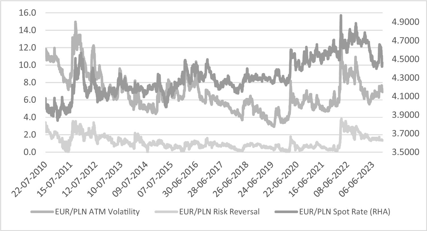
Chart 1
Spot vs ATM volatility and risk reversal on EUR/PLN market.
Source: Refinitiv.
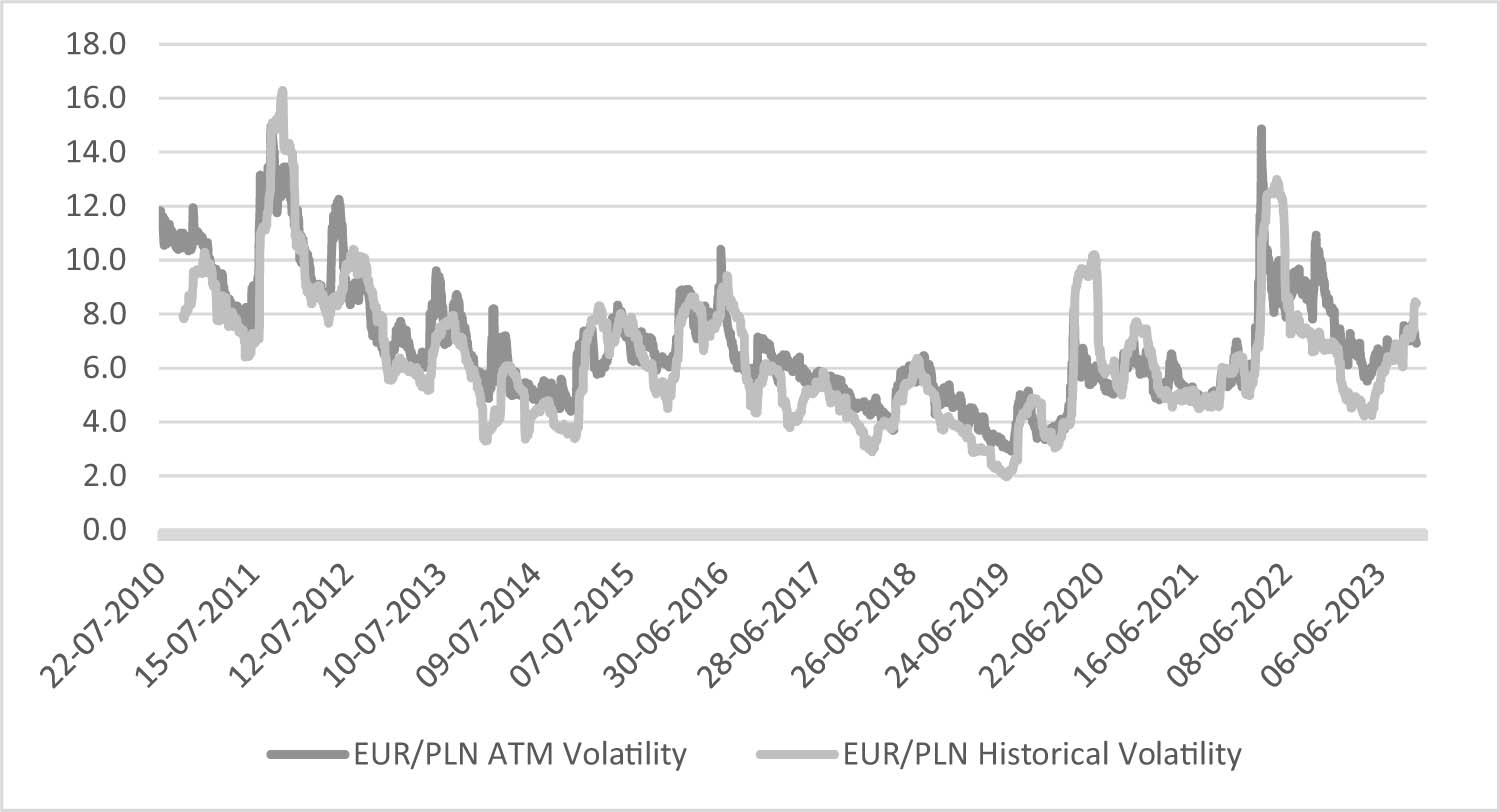
Chart 2
Implied vs historical volatility on EUR/PLN market.
Source: Author’s own calculations on the basis of Refinitiv data.
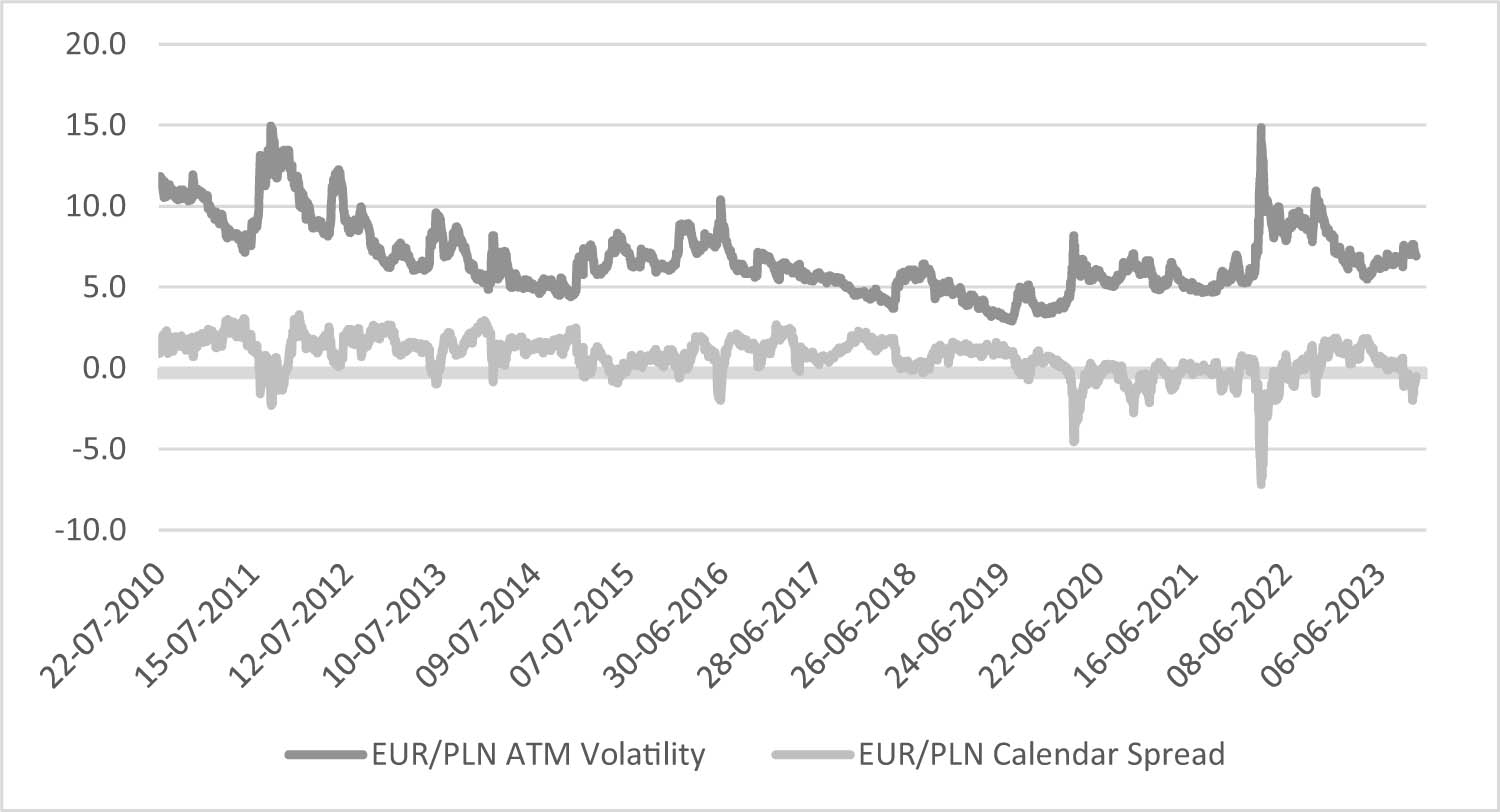
Chart 3
ATM volatility vs calendar spread on EUR/PLN market.
Source: Author’s own calculations on the basis of Refinitiv data.
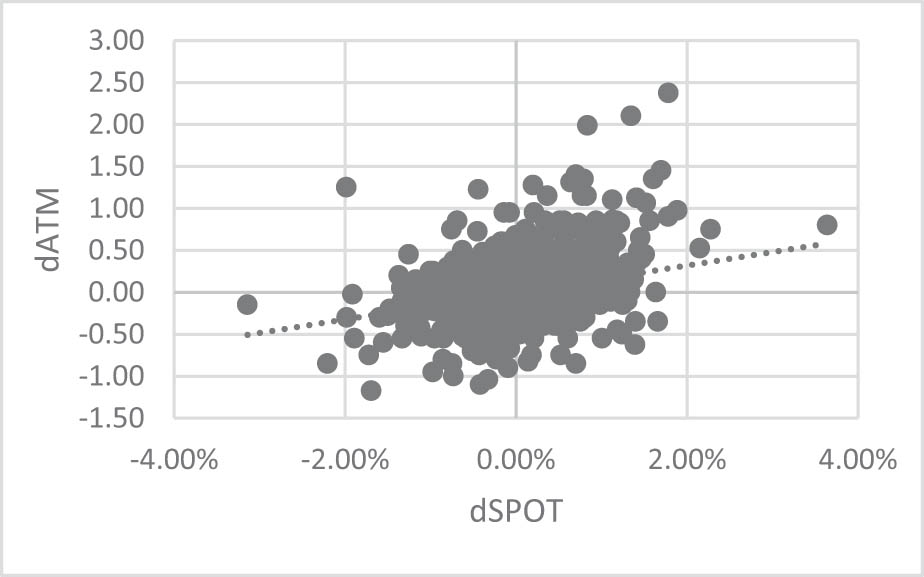
Chart 4
Plot of ATM volatility and FX spot returns.
Source: Author’s own calculations.
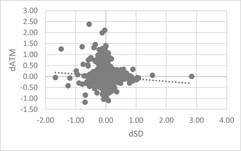
Chart 5
Plot of ATM volatility and historical standard deviation.
Source: Author’s own calculations.
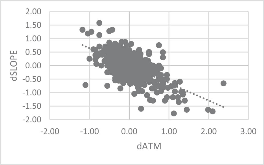
Chart 6
Plot of volatility curve slope and ATM volatility.
Source: Author’s own calculations.
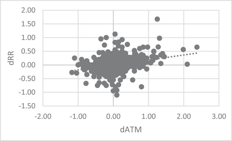
Chart 7
Plot of risk reversal and ATM volatility.
Source: Author’s own calculations.
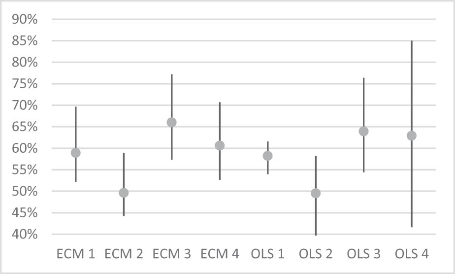
Chart 8
DQM range for the 2010–2023 period. Dot: average value, black bar: min-max for 14 annual periods.
Source: Author’s own calculations.
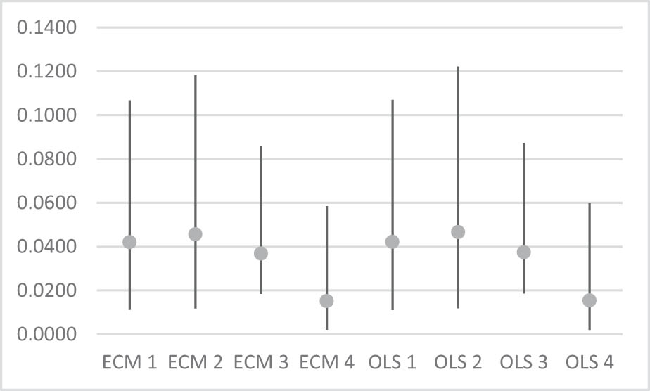
Chart 9
MSE range for the 2010–2023 period. Dot: average value, black bar: min-max for 14 annual periods.
Source: Author’s own calculations.
Table A1
Pearson correlation matrix (for daily returns).
| 1M ATM | 3M ATM | 6M ATM | 1Y ATM | |
|---|---|---|---|---|
| SPOT | 32% | 32% | 29% | 25% |
| RR | 33% | 31% | 24% | 11% |
| SD1 | 11% | 15% | 14% | 12% |
| SD2 | −7% | −9% | −10% | −6% |
Source: Author’s own calculations.
Table A2
Granger causality tests (for daily returns).
| SPOT | 3M ATM | 3M RR | 3M SD | |
|---|---|---|---|---|
| SPOT | 10.031 [0.0000]* | 33.117 [0.0000]* | 3.6827 [0.0025]* | |
| 3M ATM | 0.5771 [0.7176] | 16.916 [0.0000]* | 7.9984 [0.0000]* | |
| 3M RR | 1.5067 [0.1842] | 4.1901 [0.0008]* | 5.4973 [0.0000]* | |
| 3M SD | 0.9866 [0.4243] | 1.8946 [0.0919]* | 0.2716 [0.9288] |
*Rejection of the hypothesis about the lack of causality at 0.10 confidence level.
The table presents F-statistics for a test assuming that variables listed in the left-hand column Granger-cause variables listed in the top row of the table.
Source: Author’s own calculations.
Table A3
Stationarity tests.
| Variable | p-value for Augmented Dickey Fuller test (ADF) test | p-value for KPSS test | ADF decision – H0: I(1) | KPSS decision – H0: I(0) |
|---|---|---|---|---|
| SPOT | 0.1401 | Value p < 0.01 | I(1) | I(1) |
| 3M ATM | 0.0168 | Value p < 0.01 | — | I(1) |
| 3M RR | 0.0010 | Value p < 0.01 | I(0) | I(1) |
| 3M SD | 0.0000 | Value p < 0.01 | I(0) | I(1) |
| SLOPE | 0.0000 | Value p < 0.01 | I(0) | I(1) |
Source: Author’s own calculations.
Table A4
Residuals stationarity Engle–Granger test (full sample model)
| Model | Residual variable | p-value for ADF test | ADF value for m = 4, n = 3,284 | MacKinnon (1994) decision | Blangiewicz–Charemza (1990) decision |
|---|---|---|---|---|---|
| 1 | uhat1 | 0.0004 | −3.5194 | I(0) | Rejected |
| 2 | uhat2 | 0.0000 | −4.9595 | I(0) | I(0) |
| 3 | uhat3 | 0.0000 | −5.5724 | I(0) | I(0) |
| 4 | uhat4 | 0.0000 | −4.6977 | I(0) | I(0) |
Extrapolated critical value according to Blangiewicz–Charemza (1990) amounts to 3.88–4.17.
Source: Author’s own calculations.
Table A5
Residuals stationarity Engle–Granger test (training sample model)
| Model | Residual variable | p-value for ADF test | ADF value for m = 4, n = 2,889 | MacKinnon (1994) decision | Blangiewicz–Charemza (1990) decision |
|---|---|---|---|---|---|
| 1 | uhat1 | 0.0009 | −3.3240 | I(0) | Rejected |
| 2 | uhat2 | 0.0001 | −4.0312 | I(0) | Rejected |
| 3 | uhat3 | 0.0000 | −5.0795 | I(0) | I(0) |
| 4 | uhat4 | 0.0000 | −5.2407 | I(0) | I(0) |
Extrapolated critical value according to Blangiewicz–Charemza (1990) amounts to 4.09–4.38.
Source: Author’s own calculations.
Table A6
ECMs (full sample model).
| Model | Response variable | Explanatory variable | α 1 | α 2 | β 0 | β 1 |
|---|---|---|---|---|---|---|
| 1 | 3M VOL | EURPLN | 15.9853*** | −0.0048*** | 9.0466*** | −0.5205*** |
| 2 | 3M VOL | 3M SD | −0.1393*** | −0.0180 *** | 3.4137*** | 0.5325*** |
| 3 | SLOPE | 3M VOL | −0.6468*** | −0.0226*** | 1.0460*** | 0.0453*** |
| 4 | 3M RR | 3M VOL | 0.1813*** | −0.0399*** | −0.7478*** | 0.2750*** |
Source: Author’s own calculations.
Table A7
ECMs (training sample model).
| Model | Response variable | Explanatory variable | α 1 | α 2 | β 0 | β 1 |
|---|---|---|---|---|---|---|
| 1 | 3M VOL | EURPLN | 14.7215*** | −0.0045*** | 21.9061*** | −3.5772*** |
| 2 | 3M VOL | 3M SD | −0.1103*** | −0.0172*** | 2.9705*** | 0.5878*** |
| 3 | SLOPE | 3M VOL | −0.6029*** | −0.0248*** | 0.6832** | 0.0245*** |
| 4 | 3M RR | 3M VOL | 0.1535*** | −0.0601*** | −0.6246*** | 0.2434*** |
Source: Author’s own calculations.
Table A8
DQM for ECM models (full sample model).
| Model | Response variable | Explanatory variable | DQM (excluding zero returns) |
|---|---|---|---|
| 1 | 3M VOL | EURPLN | 58.9% |
| 2 | 3M VOL | 3M SD | 49.6% |
| 3 | SLOPE | 3M VOL | 66.0% |
| 4 | 3M RR | 3M VOL | 60.6% |
Source: Author’s own calculations.
Table A9
DQM for ECM models (training sample model).
| Model | Response variable | Explanatory variable | DQM (excluding zero returns) |
|---|---|---|---|
| 1 | 3M VOL | EURPLN | 60.7% |
| 2 | 3M VOL | 3M SD | 60.3% |
| 3 | SLOPE | 3M VOL | 73.6% |
| 4 | 3M RR | 3M VOL | 62.5% |
Source: Author’s own calculations.