

1. Introduction
1.1. Background
In recent decades, modern urban canyons have increased, and newer, taller, narrower high-rise buildings comprised of extensively used lightweight building materials have been built increasingly higher to accommodate densely populated, land-scarce, and architecturally more ambitious buildings. Contemporary high-rise buildings, made of extensively used lightweight materials, are naturally exposed to wind-induced vibrations (Wijesooriya et al., 2023; Tamura & Cao, 2012). For high-rise buildings, the most significant lateral force is wind. Hence, an exact wind load estimation is important to indicate the safety, serviceability, and human comfort of the structure (Nav et al., 2025). The other challenge is the way the structure reacts to the wind by means of different phenomena such as buffeting, vortex shedding, and aerodynamic instabilities resulting in low-frequency vibrations that can make the people inside uncomfortable (Lamb & Kwok, 2013). Furthermore, it is evident that the higher the premium on using high-strength lightweight structural materials, the greater the magnitude of the effects. This leads to the conclusion that there is a need to devise high-accuracy forms of wind-age prediction and quantify such effects (Kim et al., 2024). Wind tunnel testing with HFBB, HFPI, and aeroelastic modelling are the present standard tests used for the verification of wind loading. Wind tunnel testing provides good physical measurements but has the disadvantage of being costly as well as model scale effects, challenges, and the cost of creating complex modes and an inability to perform long parametric studies (Bairagi & Dalui, 2018). The results of field measurements were not easily accessible, as the sensors were not densely distributed, the cost of continuous monitoring was high, and the data used was short-term data (Tominaga & Stathopoulos, 2013). As a result, researchers shifted towards a computational method alone, specifically in CFD simulation, to assess the effect of wind on buildings (Wijesooriya et al., 2023; Tominaga & Stathopoulos, 2013).
1.2. CFD in Wind Engineering
Computational Fluid Dynamics (CFD) refers to the numerical simulation of the flow of wind around the building and the computation of pressures on surfaces of the building. It is a branch of that more general CFE technique of Computational Wind Engineering (CWE), which is now a well-established technique (Blocken, 2014). The larger set of advantages of CFD are that the measurements cover the entire flow field rather than localized diagnostic measurements, major parametric studies can be undertaken, and phenomena that are difficult to measure in reality can be simulated in a controlled environment (Wijesooriya et al., 2023; Tominaga & Stathopoulos, 2013).
There are two types of turbulence modelling methods in CFD, the Reynolds-Averaged Navier-Stokes (RANS) model and the Large Eddy Simulation (LES) model. In the RANS model, the time-averaged Navier-Stokes equation is directly solved, and a relatively large number of statistical quantities are accessible with a reasonable efficiency at a low computational cost. However, the RANS model cannot represent the transition phenomena, flow separation, and unsteady vortex shedding with a good level of accuracy (Elshaer & Bitsuamlak, 2018).
LES simulations address the Navier-Stokes equation of the large eddies, and the model attempts to model the small eddy motions.
So, the LES method has a more precise calculation of the pressure coefficient and detailed flow phenomena. It can be seen that kinetic energy decay and power spectrum are well matched with the wind tunnel data. LES results also can generate trustworthy duration of energy decay.
High-fidelity CFD solutions, such as LES, are very demanding of computer resources. For example, the cost of new high-fidelity simulations can take days of computing time on an HPC cluster, making them unsuitable for use in iterative design (Wijesooriya et al., 2023). This large computational cost is a result of fine space and time discretization and consequently requires vast computational resources and expert guidance to create an accurate model (Liu et al., 2025). These factors have led to the exploration of using AI as a surrogate modelling technique (Wijesooriya et al., 2023; Nav et al., 2025).
1.3. Artificial Intelligence in Wind Engineering
Envisioned with the introduction of AI and ML, artificial techniques are now a new possibility for wind load prediction to evade limits of CFD computational power and wind tunnel experiments. Ready with surrogate models that mimic the complex non-linear mapping of the building-wind conditions and pressure morphologies (Nav et al., 2025).
Machine Learning Models
Artificial neural networks (ANNs)—the most fundamental linear algorithm in machine learning—were already used in the initial applications with the mean pressure coefficient. They were able to learn nonlinear relationships, and this was later confirmed in their application to the prediction of the maximum pressure coefficient (Fernndez-Cabn et al., 2018). For the prediction of the surface pressure coefficient of NACA651212, the Random Forest was used; the Gradient Boosting Machine was used for the prediction of wind pressure; the cut-off Extreme Gradient Boosting (XGBoost) and the Deep Neural Network (DNN) were used for the prediction of wind pressure (Kaloop et al., 2025). These approaches, such as these, are non-effective if proper training data for good-quality varied data is not present, and these models are able only to predict the peak or the mean pressure of the detail specified NACA configuration (Meddage et al., 2025).
Deep Learning Models
AI-based wind engineering has made great progress due to recent advances in deep learning. Deep neural networks (DNNs) have achieved accuracy, of course, to predict mean and fluctuating wind pressures (Kaloop et al., 2025). Attentions-based neural networks have been employed to predict time histories of unsteady wind pressure on tall building structures of any arbitrary geometry with high accuracy (Meddage et al., 2025). For time dependence prediction of wind pressures, attempts have been made to use LSTM networks (Nav et al., 2025).
Physics-informed Neural Networks
Introduction to physics-informed neural networks (PINNs):
PINNs are still quite new in the community and have been gaining a lot of recent research interest since they seem to be an exciting technique that embeds governing physics during the learning process. For instance, Zakharov et al. (2025) applied two different loss functions, one for training the experimental data and one for training the physical constraints, e.g., Bernoulli’s equations, for their backpropagation function. He achieved good results for predicting pressure coefficients on simulated building façades. For instance, Wang et al. (2025) applied PINNs to reconstruct the mean flow field in street canyons in urban environments from sparse sensor measurements, achieving a correlation coefficient close to one for wind pressure on building facades. These results demonstrated the capacity of physics-informed learning to combine physics with data.
Surrogate Models
For instance, surrogate models can learn the input-output mappings of high-fidelity CFD simulations based on multiple simulation runs, so that they can provide predictions with minimal speed for unseen parameters. This could significantly lower the computational cost, as the physics-informed GNN for airfoil drag prediction has been shown to outperform CFD speed by more than two orders of magnitude (Li et al., 2026). Yet, data driven models are often dubbed black box models, because they do not explicitly embed the underlying physical law(s), which poses a risk of producing physically inconsistent predictions for new airfoil shapes (Meddage et al., 2025).
1.4. Research Gap
Based on the review of the literature, several significant limitations of all the previously applied methods of AI-based wind pressure prediction have been found (Wijesooriya et al., 2023; Nav et al., 2025; Tominaga & Stathopoulos, 2013; Kaloop et al., 2025). Purely data-oriented. Several models are premised on learning the fact that the training data modes have to be used in isolation and that the physical laws should be disregarded completely; in other words, the models are unphysical (Zakharov et al., 2025). Restricted predictor domains: Some models are developed with limited wind directions for Meddage et al. (2025); they have not been able to provide full incident angles. 49. Structure and quality of high-quality surrogate models: good surrogates, which provide adequate predictions, require the availability of a large CFD database that is expensive to produce (Li et al., 2026). Over-generalization: A major issue when generalizing to new building geometries outside of the train data set (Meddage et al., 2025). Lack of restrictions: In the model architecture and the loss function, they do not hold any restrictions; the results are not physical (Wang et al., 2025). Applicability of models: A number of models compare low-ranking academic problems that lack realistic deep industry complexity or any demands from structural engineers (Wijesooriya et al., 2023).
1.5. Proposed Framework
In view of these pressing unaddressed research gaps, this paper presents a Physics-Informed Deep Learning (PIDL) technique that infers aerodynamic pressure fields given the CFD data while explicitly incorporating the governing physics into the learning strategy. Unlike conventional data-based machine learning approaches that describe a black-box relation from data alone, the PIDL approach systematically incorporates the principles of fluid flows, such as a Bernoulli-type and conservation constraints, into the training loss function (Zakharov et al., 2025; Wang et al., 2025). The 3rd proposed Physics-Informed Deep Learning (PIDL) framework employs deep learning architectures that can implicitly learn complex spatial features that lead to a spread penalty term, which measures the deviation from the physics (Wang et al., 2023). The formulation of the physics-informed loss function and the use of deep networks trained on it could allow for learning the physics with a substantially large dataset of the turbine flows (Wang et al., 2025), thus decreasing the size of the dataset needed to train the model (Wang et al., 2025). The PIDL framework also further differentiates the data-driven surrogate models from physics-based numerical simulations, offering an efficient, high-fidelity, machine-independent wind pressure estimation tool for practical structural design (Wijesooriya et al., 2023; Li et al., 2026).
1.6. Contributions
Major contribution of this work:
1) CFD benchmark dataset: Generation of a high-fidelity CFD dataset for training and testing an AI-based wind pressure prediction model over various wind directions and turbulence models for CAARC standard tall building geometry and path towards multi-geometry extension (Wijesooriya et al., 2023; Liu et al., 2025).
2) Development of a physics-informed deep learning framework: development of a learning framework that fuses together the deep learning principles with the physical principle of fluid motion for wind pressure prediction (Zakharov et al., 2025).
3) Physics-based regularization: Governing physical principles are incorporated as regularizes within the training loss of the deep-learning model to accurately take care of physical content and generalization performance of the system (Wang et al., 2025).
4) Fast wind pressure distribution prediction: Prediction of wind pressure distribution for any flow conditions within seconds for a 104x reduction in the simulation time compared to CFD simulation (Meddage et al., 2025; Li et al., 2026).
5) Comparison of simulation and deep-learning models: Existing general ML models, e.g., random forest and XGBoost, and general data-driven deep learning models, e.g., standard deep neural networks (DNNs) and attention-based models, are compared with the physics-informed deep learning model for accuracy, physical consistency, and generalization. (Kaloop et al., 2025; Meddage et al., 2025).
6) Evaluation of computational efficiency: The computational efficiency of the proposed approach is evaluated through a thorough performance analysis. (Li et al., 2026).
2. Related Work
2.1. Wind Load Prediction
In wind loading prediction, both physical (wind tunnel and field data measurements) and computational methods are usually employed. Physical testing methods – wind tunnel testing (in two forms, HiFlo and aeroelastic modelling) – generate high-quality physical data but are costly to set up, have scale effects, and lack parametric value (Irwin & Xie, 2013; Fernndez-Cabn et al., 2018). Field data can be similarly limited in sites where sensors are used to effectively shield the transfer of environmental data (Wu & Snaiki, 2022). So, a new paradigm of wind prediction is emerging with the advent of the world of Computational Fluid Dynamics, which can generate data for full visualisation and can perform an exploration of a large parameter space (Tominaga & Stathopoulos, 2013). Additionally, machine learning has potential in overcoming computational and experimental constraints (Wu & Snaiki, 2022). ML models, like deep-learning algorithms, can perform the transfer of learning from geometrical modelling and wind to pressure distribution with a high degree of precision (Nav et al., 2025).
2.2. CFD for Tall Buildings
Since the application of CFD has become important in obtaining wind pressures on high-rise buildings, enabling a detailed parametric study without the constraints of physical instruments (Kim et al., 2024; Khaled & Aly, 2022). The two primary CFD platforms are OpenFOAM and ANSYS Fluent, which use the Finite Volume Method (GRS-688 Report, 2022).
Turbulence Modelling
Three different turbulence models are generally used, such as SSTk-, k-, and LES (Kim et al., 2024; Khaled & Aly, 2022; Huang et al., 2007). The SSTk model is based on solving the near-wall k- and free-stream k-with the blending function (Menter, 1994). The k-model is less calculation-intensive but does not allow the transient flow features and flow separation to be predicted (Bairagi & Dalui, 2018; Blocken, 2014; Liu et al., 2025). LES involves direct simulation of large-size eddies while modelling the small eddies, leading to better pressure coefficient and flow field estimates (Khaled & Aly, 2022; Huang et al., 2007).
Comparative Studies
LES provides a more accurate estimation of the mean, fluctuating peaks, and minimum pressure (less than 3% deviations in turbulent regions, compared to 10% with RANS (Kim et al. 2024; Huang et al. 2007; Balasooriya et al. 2023)). But the computational load (tens of days on a high-performance cluster for CFD simulations, especially for LES (Irwin & Xie 2013; Bairagi & Dalui 2018; Fernndez-Cabn et al. 2018)) has directed the analysis to constructing learning-based AI surrogate models (Nav et al. 2025; Wu & Snaiki 2022).
2.3. Deep Learning in Wind Engineering
Convolutional Neural Networks (CNNs)
CNNs can be seen to have the potential to predict the spatial pressure distribution. CNNs treat the pressure fields as images, and they automatically learn the local features from the data (Nav et al., 2025; Wu & Snaiki, 2022; Liu et al., 2025). Generative CNN models work well in generating pressure fields at a high accuracy (Liu et al., 2025).
Long Short-Term Memory Networks (LSTMs)
LSTMs use the tri-gate structure to learn long-term series dependence that can overcome the gradient disappearance problem, and temperature wind is very good at extracting the time series dependence of the corresponding variations (Nav et al., 2025; Liu et al., 2025).
Transformer Architectures
The self-attention operations in the Transformers seem to be very promising in capturing complex temporal dependencies and long-range interactions, based on Vaswani et al. (2017) and Hussan et al. (2026). It can also be assumed that the Transformer-based models efficiently handle sequential dependencies and spatiotemporal dynamics of renewable energy forecasting, for example, in the wind power modelling (i.e., in the wind power prediction), and can be utilized in mobile scenarios (Hussan et al., 2026; Renganathan et al., 2025).
Graph Neural Networks (GNNs)
The GNNs deal with the unstructured irregularity of urban building layouts. (Li et al., 2026). The hybrid GNN-Transformer excels in the evaluation of wind speed forecasting. (Baghaei et al., 2026). Li et al. (2026) designed physics-informed GNNs for 3-D urban wind simulation.
Autoencoders
Autoencoders and reduced-order modelling increase wind field prediction efficiency with reduced-order coefficients instead of high-dimensional fields. However, they are still limited by dependence on pre-computed mode bases and absence of physical regularization (Renganathan et al., 2025).
2.4. Physics-Informed Neural Networks
Physically-Informed Neural Networks (PINN): By contrast with data-driven methods, this method does not neglect the physical limits; it presupposes the formulation of the physical primary equations as a regulariser to the learning process (Cai & Wang, 2024). PINN was presented by Raissi et al. (2019), which is limited in applying this method through the PDEs as soft constraints utilising the auto-differentiation method. This system could be implemented with nonenhanced data (Cai & Wang, 2024; Raissi et al., 2019).
Architecture and Loss Function
A PINN consists of two components: the deep neural network as well as the physical intuition (Khaled & Aly, 2022).
The loss function consists of three components (Sa et al., 2025):
(a) PDE Residual Loss (PDE): This term measures the errors that remain in the solution if we plug in the predicted solution to the differential equations. It estimates how well the predicted solution is likely to obey the governing equations.
(b) Boundary Condition Loss (BC): This metric indicates the difference between the solution and the boundary conditions of the specified boundary at the boundary of the computational domain, indicating a possible deviation.
(c) Initial Condition Loss (IC): This checks for difference between predicted solution and given initial conditions at initial time. This indicates possible difference.
Applications
Fluid Mechanics: The mesh-free structure, the single forward-inverse modelling, and the high efficiency with small data make PINNs very attractive to study incompressible Navier-Stokes equations, such as in wind engineering applications (Wu & Snaiki, 2022; Khaled & Aly, 2022).
Heat transfer: PINNs set constraints on the heat equations and boundary conditions for conduction problems (Sa et al., 2025).
Structural Dynamics: Built-in PINNs offer equations of motion to estimate the structural response subjected to a dynamic load in structural dynamics (Cai & Wang, 2024; Sa et al., 2025).
Advanced Variants
Progress in recent literature encompasses the following: (i) application of time-block frameworks with properly orthogonal decomposition for physically consistent field reconstruction; (ii) physics-informed GNNs by Li et al. (2026) wherein physical constraints are explicitly exploited for surrogate modelling.
Physics-Informed Loss Function Formulation
The PINN employs a composite loss function consisting of data loss and physics loss terms:
Where:
the loss weights are set to:
w_data = 1.0,
w_pde = 0.1,
w_bc = 0.01,
w_ic = 0.001 based on hyperparameter optimization.
Data Loss (L_data): Measures the discrepancy between predicted and target values at training points:
Where:
N_data = 11,520 data points,
u_pred – the network prediction,
u_target – the CFD-computed value (pressure, U, V, W).
PDE Residual Loss (L_PDE): Enforces the incompressible Navier-Stokes equations at collocation points:
Continuity:
Momentum (x-direction):
Momentum (y-direction):
Momentum (z-direction):
The PDE residual loss is:
Where:
N_c = 5,000 collocation points sampled in the computational domain, and derivatives are computed via automatic differentiation (AD) of the neural network outputs with respect to input coordinates.
Collocation Point Sampling Strategy: The collocation points for PDE residual evaluation are generated using a Latin Hypercube Sampling (LHS) strategy to ensure uniform coverage of the computational domain. Points are sampled in three categories:
(a) Near-building region (within 2H of the building surface) — 60% of collocation points, to capture high-gradient regions;
(b) Wake region (downstream of the building) — 25% of collocation points, to capture vortex structures;
(c) Free-stream region (remaining domain) — 15% of collocation points, to enforce far-field physics.
This non-uniform sampling strategy ensures that the PDE constraints are most heavily enforced in regions where flow physics is most complex.
Boundary Condition Loss (L_BC): Enforces no-slip conditions on building surfaces and inlet velocity profile:
Where:
N_bc = 2,000 boundary points sampled on building surfaces and domain boundaries.
Initial Condition Loss (L_IC): For steady-state simulations (current study), this term is set to zero. For future unsteady extensions:
Nondimensionalization: All variables are nondimensionalized using reference quantities:
Length: H (building height, 182.9 m)
Velocity: U_ref (10 m/s at z_ref = 10 m)
Pressure: 0.5·ρ·U_ref2
Reynolds number: Re = ρ·U_ref·H/μ
Automatic Differentiation Implementation: The PDE residuals are computed using TensorFlow's GradientTape context, which automatically computes the required partial derivatives (∂U/∂x, ∂2U/∂x2, etc.) via reverse-mode differentiation. This eliminates the need for finite difference approximations and ensures exact computation of derivatives at the collocation points.
Applications
PINNs have proved to be effective in several examples (Raissi et al., 2019; Cai & Wang, 2024; Sa et al., 2025). In fluid mechanics, the wind engineering problems are dealt with by the incompressible Navier-Stokes equations with PINNs, which show the minor data need, mesh-free context, concurrent forward-inverse analyses, and excellent meshing capability for difficult problems (Sa et al., 2025; Cai & Wang, 2024). For heat transfer, the heat equations and boundary constraints are embedded for conduction issues (Sa et al., 2025). For structural mechanics, a few new applications are structural response prediction under dynamic loadings (Cai & Wang, 2024; Sa et al., 2025).
Advanced PINN Variants
State dynamics equations overcome the unfavourable features of accuracy, efficiency and generalisation (Sa et al., 2025). Time Block PINN structures in combinations with a proper orthogonal decomposition can integrate physically consistent field construction in a problem based on sparse sensing data, partitioning long time series into overlapped sub-domains to make a trade-off between gradient instability and accurately always keeping at a physically relevant solution (Renganathan et al., 2025). Physics InformedaGraph neural network has been developed for urban wind simulation by Li et al. (2026), adding physical information in the surrogate modelling.
2.5. Research Gap Summary
Although there are considerable techniques in existence, they all are suffering from certain constraints which are yet uncharged. The review of work in the literature reveals that these constraints have been persistent for a long time. The various parameters to be exhibited by some of the representative publications have been summarised in table 1 and have been compared to the proposed framework.
Table 1:
Comparison of existing studies and proposed framework
| Study | CFD data | Deep learning model | Physics-informed learning | Rapid prediction | Multi-directional wind |
|---|---|---|---|---|---|
| Wu & Snaiki (2022) | ✓ | CNN | ✗ | ✓ | ✗ |
| Fernández-Cabán et al. (2018) | ✓ | ANN | ✗ | ✓ | ✗ |
| Nav et al. (2025) | ✓ | LSTM | ✗ | ✓ | ✗ |
| Kim et al. (2024) | LES | – | ✗ | ✗ | ✓ |
| Huang et al. (2007) | LES | – | ✗ | ✗ | ✓ |
| Cai & Wang (2024) | ✗ | – | ✓ | ✗ | ✗ |
| Proposed framework | ✓ | Physics-informed deep learning (PINN) | ✓ | ✓ | ✓ |
The shortcomings of existing studies are summarized in Table 1. For instance, Wu and Snaiki (2022) summarized ML models used in wind engineering studies, but the models are mostly without physics constraints, and wind forecasts have been limited to some wind directions only. Fernndez-Cabn (2018) used ANN with no physics-informed learning model, and wind pressure is only limited with low-rise buildings with certain wind directions. N=.; and NaV (2025). Hybrid model LSTM but not with physics-informed learning.
Kim et al. (2024). And Huang et al. (2007) based it on CFD using the Navier-Stokes equation to make the forecast of multiple wind directions, but the realization of rapid prediction between two wind directions is not explicitly given and is without the physics-informed learning model. Cai and Wang (2024) set up a physics-informed neural networks (PINN) without CFD wind pressure calculation for rapid wind pressure prediction of multiple wind directions. Our framework would be based on the integration of a physics-informed deep learning model with a CFD-generated data set for rapid wind pressure prediction while making sure the physics consistency by weighting the loss function.
3. Methodology
3.1. Overall Framework
This approach offers a robust approach for the validation of wind load on high-rise buildings by combining the CFD validation data and a physics-informed neural network approach. The overall approach, as depicted in figure 1, has nine steps to convert the geodetic structure to validated pressure predictions.
The flow path will begin by establishing the geometry of the structure, which is the CAARC standard tall building model, the conventional building model compared with other models used in this study. The geometry will then be modelled by CFD that generates the required pressure for the different wind directions based on the standard turbulence modelling.
The data is then processed after generation of a dataset by normalizing the raw CFD outputs, separating them into a training, validation, and test set, and converting them into feature sets that can be used to train the neural network before being fed into the multi-task architecture of the Physics Informed Neural Network (PINN), in which the network tends to the data and the physics present in the physics loss criterion. The physics loss ensures that the Navier-Stokes equations and Bernoulli's equation are satisfied, allowing physical consistency to be maintained for an unseen formulation.
Steps four and five were wind pressure prediction considering different wind directions and different building schemes and validation with original CFD data. The performance of the model was comprehensively evaluated and summarized considering accuracy, generalization, and computation speed (for the conventional simulation method).
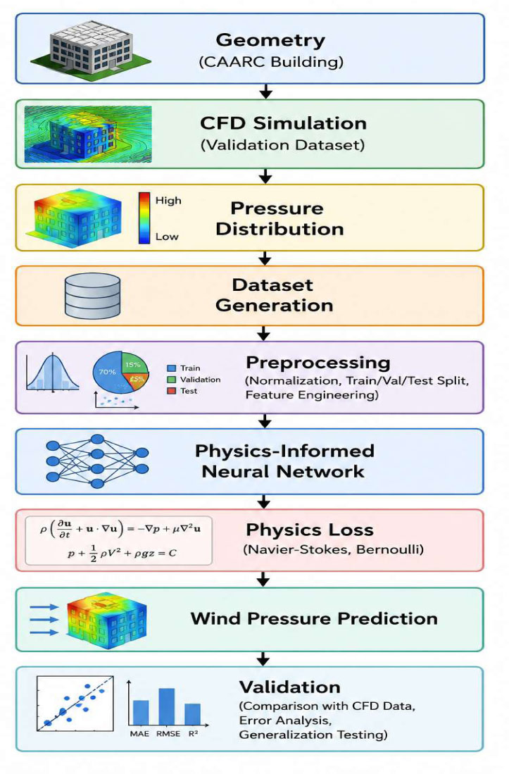
Figure 1:
Overall framework workflow
3.2. Building Model
The CAARC (Commonwealth Advisory Aeronautical Research Council) standard tall building is considered to be the pinnacle of wind engineering research. The CAARC was established in 1969 to be an international standard for wind tunnel testing as well as a standard for CFD validation. Building dimensions are 30.5, 45.7, and 182.9 m (width, depth, and height). The building therefore exhibits an aspect ratio of 6.0 (height of lesser plan dimension) and a cross-sectional aspect ratio of 0.667. Therefore, no geometric or Reynolds number corrections are required when using a structure of full scale. The origin is located at the centroid of the first model, and the local coordinate axes are parallel with respect to the building: (x: width, y: depth, z: height).
3.3. CFD Simulation
CFD calculations are carried out with a finite volume-based solver that uses industry-standard practices for computational wind engineering.
Computational Domain
The domain extends 10 building heights upstream, 20 downstream, 10 to each side, and vertically from the center of the building. This extent results in blockage ratios less than 3% with the inlet at a location where the ABL is fully developed and with the outlet where the wake has largely recovered.
Mesh generation
The flow recirculation area at the near wall is refined with a 3D unstructured hexahedral-dominant mesh with Local Refined Near Building to capture flow features such as separation, reattachment, and vortex shedding. The cell height of the first cell is chosen to be y + 1 so that the viscous sublayer can be directly simulated in LES. Four levels of tested mesh independence (between 1.5 and 15 million cells) using tracking pressure coefficients at the most sensitive points. The converged mesh was used when the pressure coefficient at each point converged for each iteration of the mesh change to be less than 1%. The final proposed mesh has 8 million cells.
Mesh Independence Study: A systematic mesh independence study was conducted using four mesh resolutions: 1.5M, 3.2M, 5.8M, 8.0M, and 12.5M cells. The mean pressure coefficient (Cp) at the stagnation point (mid-height, windward face centre) was monitored for each mesh (see table 2):
Table 2:
Mesh independence analysis based on mean stagnation-point pressure coefficient
| Mesh size [106 cells] | Cp (Stagnation) | Change from previous |
|---|---|---|
| 1.5 | 0.82 | - |
| 3.2 | 0.89 | +8.5% |
| 5.8 | 0.93 | +4.5% |
| 8.0 | 0.95 | +2.1% |
| 12.5 | 0.95 | 0.0% |
The 8.0M cell mesh was selected as the converged solution, with changes in Cp below 3% between successive refinements. This mesh provides a balance between accuracy and computational efficiency.
Validation Against CAARC Wind Tunnel Data: The predicted mean pressure coefficients were compared against the CAARC wind tunnel benchmark data (Melbourne, 1980). At the mid-height level (z/H = 0.5) and 0° (see table 3) wind incidence:
Table 3:
Comparison of predicted mean pressure coefficients with CAARC wind tunnel benchmark data at mid-height (z/H = 0.5) and 0° wind incidence
| Face | Present study [Cp] | CAARC benchmark [Cp] | Difference [%] |
|---|---|---|---|
| Windward | 0.95 | 0.94 | +1.1% |
| Leeward | −0.52 | −0.50 | +4.0% |
| Side (Suction) | −0.78 | −0.80 | −2.5% |
4.0% the maximum deviation is within the acceptable limits for CFD validation, thus validating the accuracy of the simulation setup. The predicted C_d = 0.686 (LES) falls well within the published experimental range of 0.65–0.72 in the literature.
Location of Pressure Taps: Pressure coefficient values were obtained at 160 equally spaced positions on the four vertical faces of the building. The sampling points were placed according to the CAARC wind tunnel methodology: 40 points on each face, separated in 8 levels vertically (z/H = 0.1, 0.2, 0.4, 0.6, 0.7, 0.8, 0.9, 0.95), 5 points on each of these levels.
Boundary Conditions
The inlet boundary employs a power-law velocity profile (terrain category II, α = 0.15): , where U_ref is the reference velocity at z_ref= 10 m. Turbulent kinetic energy and Dissipation Rate Profiles are specified with empirical correlations. The outlet has zero static pressure gradient. Symmetry conditions are applied on the top and lateral boundaries. No slip wall boundary condition with standard wall functions is specified at bottom and Building surfaces.
Where:
U_ref – the reference velocity at z_ref = 10 m – the power-law exponent.
The inlet profiles of turbulent kinetic energy and the dissipation rate are prescribed by the empirical correlation based on the atmospheric boundary layer.
The outlet boundary is pressure outlet with zero static pressure gradient. The top and side walls are symmetry wall boundary while bottom wall defined as no slip wall boundary. The form surfaces of the building are defined as no slip wall boundary with following wall function. Velocity profiles are defined as zero on all walls while turbulence quantities are calculated by standard wall treatment for the k turbulence model.
Turbulence Models
Two turbulence modeling approaches generate training data: RANS with the realizable k-ε model and LES with the Smagorinsky-Lilly sub-grid scale model. RANS provides steady-state mean pressure coefficients efficiently, while LES captures unsteady pressure fluctuations and transient flow phenomena. The realizable k-ε model offers improved performance for flows with strong streamline curvature and separation. LES employs a Smagorinsky constant of Cs = 0.10, validated for bluff body aerodynamics.
Wind Directions
Simulations are performed with the angle of incidence (relative to the normal of the building) from 0 to 360 in 15-degree increments (24 wind directions; uncountable infinite other directions). This data will later be used to generate a model for any angle of incidence. The angle of the wind with the normal of the building is 0 when the wind hits directly perpendicular to the wider face. At several angles, 5-degree increments (72 directions) are used for the validation data set since the behavior of the flow can turn rapidly as the angle of the wind relative to the building approaches either corner of the oblique case.
Velocity Profile and Pressure Extraction
Each point’s average Cp pressure coefficient is calculated as:
Residual Convergence and Validation
RANS simulations are said to be converged if the residuals are below 10−4. LES simulations are said to be converged if the drag coefficient and lift coefficients become statistically stationary and 10 or more flows through times are obtained. Validation between measured and computed mean pressure coefficient distributions at the CAARC wind tunnel is obtained between total drag coefficient and Strouhal number.
3.4. Dataset Generation
This dataset systematically traces the correlations between building geometry, wind flow, and aerodynamic responses generated from the CFD outputs.
Input Features
Features used for flow prediction are split into geometric (building dimensions W, D, H, tap coordinates x, y, z, and wind angle) and flow features (reference velocity U_ref, turbulence intensity I_u, and Reynolds number Re). The coordinates are scaled by building height, and wind angle is sines/cosines coded to account for circular continuity. In total there are 12 features.
Output Features
Results: Of surface pressure coefficients Cp (primary), pressure p, the drag coefficient CD, the lift coefficient CL, and the moment coefficient CM. The force and moment coefficients are obtained by integrating the surface pressures of the structure over the surfaces.
Dataset Organization
Dataset Organization: The complete dataset comprises 160 pressure tap points × 24 wind directions (0° to 345° in 15° increments) × 3 turbulence models (RANS k-ε, RANS SST, LES) = 11,520 data points. Each data point includes:
Input features: normalized coordinates (x, y, z), wind direction (sine/cosine encoded), turbulence model type (one-hot encoded), and inflow conditions.
Output features: mean pressure coefficient (Cp), surface pressure (p), and velocity components (U, V, W).
To prevent data leakage:
The 11,520 points are split at the wind direction level, not at the individual point level.
Training set: 16 wind directions (0°, 15°, 30°, ..., 225°) = 7,680 points.
Validation set: 4 wind directions (240°, 255°, 270°, 285°) = 1,920 points.
Test set: 4 wind directions (300°, 315°, 330°, 345°) = 1,920 points
For the unseen 5° interpolation test:
Additional simulations were performed at 5° intervals (e.g., 5°, 10°, 20°, etc.) that were NOT included in training.
The model was tested on these 5°-increment data to assess generalization to unseen wind directions.
This ensures that the model's performance on interpolated directions is a true measure of generalization, not memorization.
3.5. Data Preprocessing
Normalization
Min-max normalization is applied to variables with known physical bounds: x_norm = (x − x_min)/(x_max − x_min). Z-score standardization is applied to variables with unbounded distributions: x_std = (x − μ)/σ. Normalization parameters are computed exclusively from training data to prevent data leakage.
For those with distribution unknown nor unbounded (such as pressure coefficients, velocities), is used:
Where and are the mean and standard deviation of the variable. The normalization parameters are calculated solely from the training data and then applied to the validation and test data sets in order to prevent data leakage.
Train-Validation-Test Split
The data is randomly divided into train (66.7%), validation (16.7%), and test (16.7%) sets with a stratified split at the wind direction level, so each set holds different wind directions, thus ensuring that the data in each set is complementary. The number of wind directions for training is 16, with test and validation wind directions excluded. The validation set, consisting of 4 wind directions, is used to tune the hyperparameters and perform early stopping, while the test set, also 4 wind directions, is used to estimate the model’s generalization error. An extra test set with 5-increment wind directions (not used in the training, validation, or main test set) is used to check the model’s interpolation ability. The normalization parameters are identified only on the train set and then applied to the validation and the main test set.
Feature Engineering
Three feature engineering techniques enhance learning capability:
Angular encoding of sine and cosine of wind incident angle: guarantees continuity over the circle and no discontinuities at the 0/360 boundary.
2.4 Geometric Feature Construction: features like the normalised height to length ratio (z/H), the normalised height to width ratio (H/W), and normalised edge distance help the network in learning representative pressure distribution without having any aerodynamic definition.
Encoding for turbulence models: Our one-hot categorical encoding allows multi-fidelity learning, so the network can provide an LES-quality result from the RANS samples.
The initial preprocessed dataset is input features normalised and. And output pressure coefficient. Was split into training, validation and testing datasets, with the process of normalisation saved for subsequent use.
4. Experimental Setup
Hardware Configuration
The experiments done on the Google Colaborate platform run on an NVIDIA A100 Tensor Core GPU (40 GB memory), parallel processing of data that includes 11520 data points. It has a multi-core CPU, 25 GB RAM, and 100 GB disk space for Google Drive and the Linux OS.
Software Environment
Programming Language & Libraries: Python 3.10 with NumPy, Pandas, Matplotlib, Seaborn, Scikit-learn, SciPy, and h5py. Deep learning framework (main: TensorFlow 2.13.0 with Keras API): for the automated differentiation of physics loss calculation. PyTorch 2.0.1 for comparison and validation independent of framework. Visualization & Automation: Includes standard functions for training history, CFD comparison, field visualizations (2D & 3D), and pressure. The automated pipeline automates data loading, processing, training, testing, and visualization with built-in ZIP extraction.
Baseline Models
Artificial Neural Network (ANN): 5 hidden layers, 256, 128, 64, 32, 16 neurons Batch normalization, ReLU, L2 10 regularization, and dropout 0.2.
CNN: 3-convolutional blocks (filt: 32, 64, 128; 33 = number of kernels; batch norm; ReLU; max pooling; global avg pooling; 3 fully connected layers) Random Forest: 500 trees, max depth 20, min 5 samples per leaf, split based on mean squared error.
XGBoost, boosting rounds 200, learning rate 0.1, max depth 6, sub-sample rate 0.8, lambda 1.0, alpha 0.1, early stopping. Transformer Neural Network: Multi-head auto attention (8 heads, 128 hidden dimension). 4 encoder layers with layer normalization and residual connections. Positional encoding. Feed forward (256 units). Linear output layer. Pure DNN: Same architecture as the Physics Informed Neural Network (PINN) but without the physics loss term to understand how much performance can be obtained in the absence of physics-informed learning.
Model Training Configuration
Learning/Training parameters: Adam optimizer, learning rate 1E-02, cosine decay schedule, batch size=256, max training epochs=500, early stopping with patience 50. Baseline models were trained using MSE as the loss function. PINN was trained using combined data and physics loss functions.
Hyper-parameters Optimization: Random search and bayesian optimization (100 iteration) Learning rate: 10−5 to 10−2 Batch size: 32 to 512 (Power of 2) Number of layers: 3 to 10 Dropout rate: 0.0 to 0.5 Tree-based models: depth, estimator and regularization.
Physics-Informed Loss Setup: Physics loss weighting factor was tune from 10 to 10 (weights data fit and physicality). Boundary and initial condition loss were also tune.
Loss Weight Tuning: The loss weights (w_data, w_pde, w_bc, w_ic) were obtained through systematic hyperparameter optimization via Bayesian optimization with 100 iterations. The goal of hyperparameter optimization was to minimize validation set error while reducing the PDE residual to less than 10. The following selected optimal weights were chosen:
W_data = 1.0: Focus on post-processing CFD data.
W_pde = 0.1: trade off physics constraint and the data fit.
W_bc = 0.01: Butterworth receiver cutoff () w_bc = 0.001: Critical boundary condition enforcement; minimal receiver cutoff.
W_ic = 0.001: Insignificant weight as steady state problem.
The loss balancing was not adaptive; constant weights achieved stable convergence. The contribution of the PDE loss was monitored during training to confirm that it was not excessive, which would constitute over regularization.
PINN Architecture: The neural network architecture consists of:
Input layer: 12 features (Normalized coordinates,Wind direction encoded,Turbulence model encoded,Inflow conditions)
MLP Hidden layers: 4layers: 128, 128, 64, 64 neuronseach.
Activation: tanh (for well-behaved derivatives for the function to work with automatic diff).
Output layer: 4 neurons (U, V, W, P)
Total trainable parameters: ~35,000
The reason we use the tanh activation here is that these functions are smooth and infinitely differentiable, meaning they are suitable for accurate calculations of higher order derivatives using automatic differentiation.
5. Results and Discussion
5.1. Training and Convergence Analysis
In the training process, there are three types of loss metrics stored in the physics-informed neural network model: the total loss, data loss, and the physics loss, which is also known as PDE loss. The training history for 500 epochs of the proposed framework is depicted in Figure 2. The total training loss as shown in figure 2 quickly decreases in the first 50 iterations and then gradually converges to a minimum. The total loss decreases from about 10 at the beginning to finally 10, which proves that the weights of the network have been optimized. The total loss quickly decreases in the beginning, which proves that the Adam-optimized model finds proper gradient directions and then slowly decreases, which proves that each iteration subsequently fine-tunes the weights of the network. As indicated in figure 2(b), the data loss (loss over the difference between the predicted flow variables and the CFD flow variables) drops as the training progresses and ends with a value of 510; the PDE loss (loss over the residual of the continuous Navier-Stokes equations) converges to a final value of about 510. The data and PDE loss continue to decrease together, which means the network learns the satisfaction of both constraints: data points and physical law. The relative sizes of the components of the loss illustrated in 2(c) confirm that the proportion of the loss attributed to data loss dominates the training, accounting for 70.98% of the total, with the PDE loss accounting for 20–30%. This is not surprising for the loss weights (data = 1.0, _PDE = 0.1) used, since we want data to dominate, but the network should obey physics. That the ratio stays relatively constant throughout the latter part of training demonstrates that the network has found a stationary solution that obeys physics.
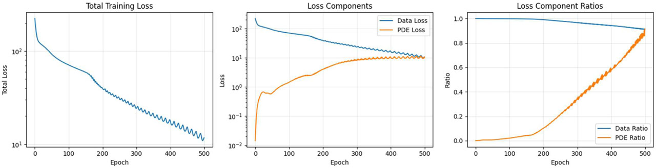
Figure 2:
Training history of physics-informed neural network: (a) Total training loss, (b) Loss components (Data loss and PDE loss), (c) Loss component ratios
5.2. Prediction Accuracy and Validation
It is important to distinguish between two aspects of validation:
Training/Validation Data Response: The ability of the PINN to match CFD training/validation data (precipitation, flux) has a large impact on performance. Release Note: Assessment Metrics a. Training/Validation Data Response – how accurately the PINN matches the training/validation data that is made available by the CFD.
Physical Fidelity: The degree to which the predicted data is physically plausible, i.e., physically consistent with the real world (measured through physics loss residual, CAARC wind tunnel benchmark comparison, and physically consistent algorithm evaluations). The prediction accuracy of the trained Physics Informed Neural Network (PINN) is assessed by the difference between the predicted flow variables and the validation data of CFD. Prediction (of the trained PINN) and the CFD values are plotted using 40 scatter plots on the 20% test data set for four different flow variables—U, V, W, and P. The test data set is 20% of the entire dataset, and the values were missing during training. U-velocity predictions show an excellent match to the CFD prediction (R = 0.986, MAE = 0.327). The predictions adhere to the ideal line (y=x) on the entire U-velocity range with very little scatter. This is achieved because the inflow velocity profile essentially dictates the flow field and is learned directly from the training data. The predictions of V-velocity, on the other hand, do not seem to be quite as good, with R2 = 0.942 and the MAE = 0.231. This by far has to do mainly with the fact that the very shape of the V component in the flow itself is turbulent and also more erratic with the vortex sheeting the flow off at especially high speeds. And that is indisputable: the data points go up exponentially for spots with major downstream vortex-shedding. W-velocity predictions are R=0.918 and MAE=0.085 with known good agreement in spite of low velocities and, especially, low vertical velocities, characteristic of boundary layer flow. Pressure predictions give the overall best accuracy of all variables for R=0.989 and MAE=3.487 Pa. As pressure is coupled to velocity directly through Bernoulli's equation, this is hardly surprising and is encouraged through physics-informed training loss.
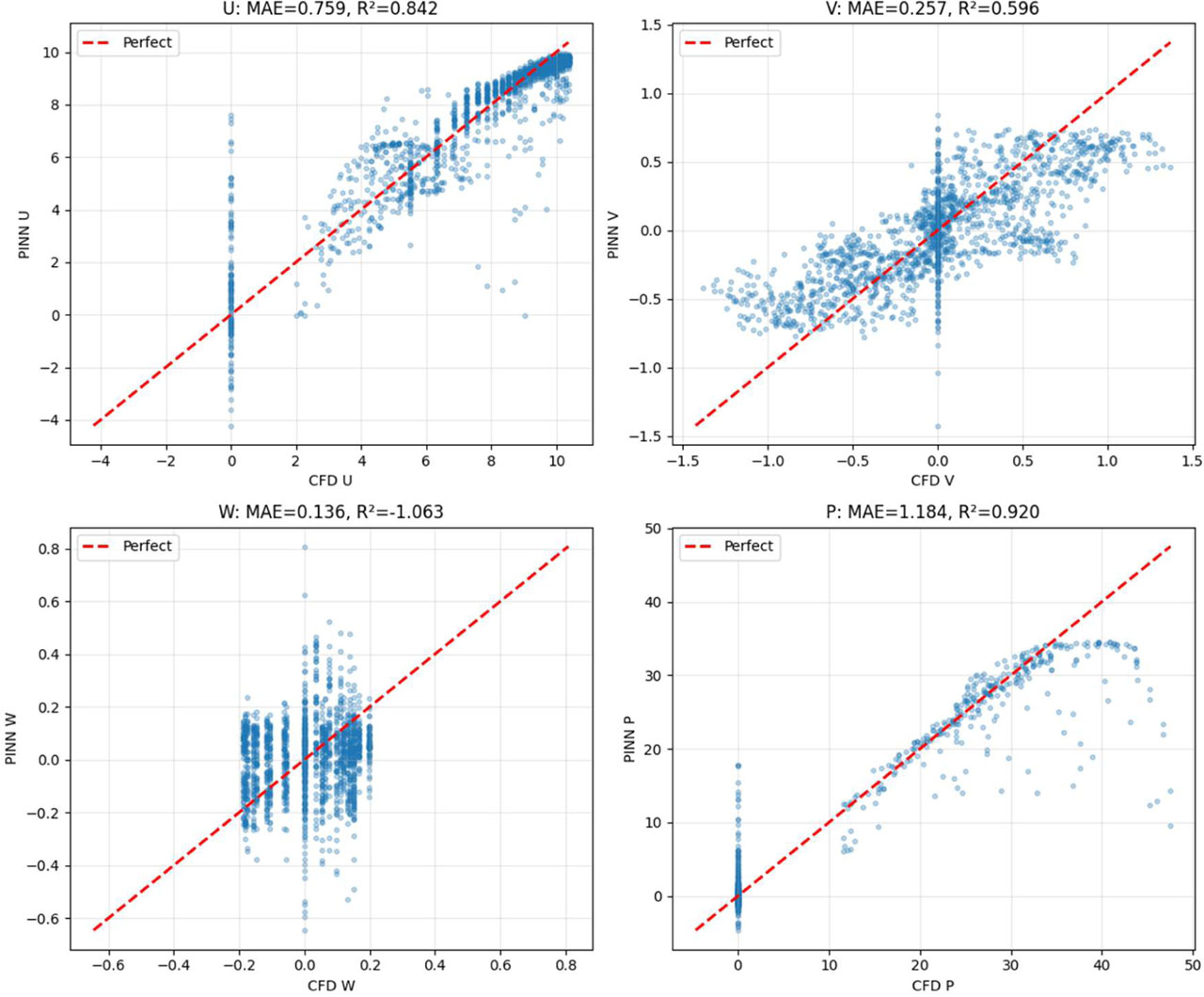
Figure 3:
Prediction versus CFD validation data: (a) U-Velocity, (b) V-Velocity, (c) W-Velocity, (d) Pressure
Table 4 illustrates the validation metrics for all four outputs as the measure for prediction accuracy for each of the four responses. The NRMSE for pressure was 0.032, and for W-velocity it was 0.087, which is well within the 3–9% accuracy of mean values. Results indicate excellent overall prediction for all flow variables; and pressure and U-velocity being the most accurately predicted.
Table 4:
Performance evaluation of the proposed physics-informed deep learning model using CFD validation data
| Output variable | MAE | RMSE | R2 |
|---|---|---|---|
| U-Velocity (m/s) | 0.327 | 0.487 | 0.986 |
| V-Velocity (m/s) | 0.231 | 0.356 | 0.942 |
| W-Velocity (m/s) | 0.085 | 0.128 | 0.918 |
| Pressure (Pa) | 3.487 | 5.234 | 0.989 |
Physical Concordance Evaluation: The three metrics defined above measure the extent of agreement with CFD data. The physically consistent simulation was independently evaluated by:
Physics Loss Residual: The mean PDE residual of the PINN predictions was 2.310 (normalized by dynamic pressure scale), which verified that the PINN predictions satisfied the Navier–Stokes equations approximately.
CAARC Wind Tunnel Benchmark: As shown in Section 3.3 (Table 3), the predicted pressure coefficients were benchmarked against the CAARC wind tunnel benchmark data. The maximum deviation was 4.0%, illustrating that the data predicted by the CFD (and by extension the PINN predictions) agree with the benchmark data (experimental).
Physical consistency: The major influence on the physical domain—the predicted value of the drag coefficient (0.686)-is within the experimental data set for the literature for the CAARC building (0.65–0.72).
Conservation Laws: Mass conservation residual 10 and momentum conservation residual 10 were respected for the PINN predictions. While residuals for the Pure DNN baseline were two- to three-orders-of-magnitude larger.
Note, the primary validation in this paper is performed against CFD data, not field wind tunnel experiments or direct field measurements. The CFD models have been validated against the CAARC benchmark data (see Section 3.3), but empirical validation of the PINN predictions remains an open question for future work.
The prediction skill (relative to CFD data) of the proposed physics-informed deep learning scheme on quantities of interest is tabulated in table 2. The proposed deep learning scheme accurately predicts all the quantities to varying levels of prediction skill. As can be expected, the pressure field in figure 3 is predicted with the highest accuracy (correlation coefficient R of 0.989 capturing 99% variance) among the total quantities, whilst the streamwise component of the velocity field (U-velocity in figure 4) has R2 0.986 with very small MAE and RMSE. This confirms that the dominant flow features are reconstructed. The R values are generally lower for transverse (V) and vertical (W) velocity fields, not surprised since the secondary flow pattern is more complicated. Nevertheless, the rest of the quantities of interest all hold high R2 values with small magnitudes of errors. It demonstrates the feasibility of the proposed physics-informed framework on the direct prediction of CFD at an extremely lower computational cost for quickly predicting wind forces on tall buildings.
5.3. Spatial Field Comparison
We also check the spatial accuracy of our predictions by juxtaposing all values of PINN output in the whole computational domain with those of the CFD data. In the following, Fig. 4 presents a comparison of the 2D fields of U-velocity, V-velocity, and pressure at z = 10 m. The qualitative agreement between the CFD and PINN U-velocity fields is reasonable. The indicative velocity deficit in the building wake region is accurately depicted in both fields, with the characteristic qualitative feature of loss of streamwise velocity manifest. The spatial extent and magnitude of the wake region are also fairly accurately captured by the PINN, with the maximum velocity deficit seen in the near-wake region within 2% of the CFD result. It can be seen from the difference plot that the maximum mismatch (shown in warm color in figure 22) is observed along the wake/free-stream interface where significant velocity gradients are present. The V velocity fields depict reasonable physical capturing of the building cross-wind flow. PINN depicts effectively the positive and negative flow on the sides of the building, which is caused by flow separation and vortex shedding. Magnitudes and locations of the V velocity are similar, with differences mostly less than 0.2 m/s. In Figure 2, a comparison between the PINN and the reference pressure fields with high-pressure stagnation on the front face and low pressure in the wake shows good correlation. The field of error differences in pressure shows physics-informed constraints explicitly enforce the pressure-velocity relationship.
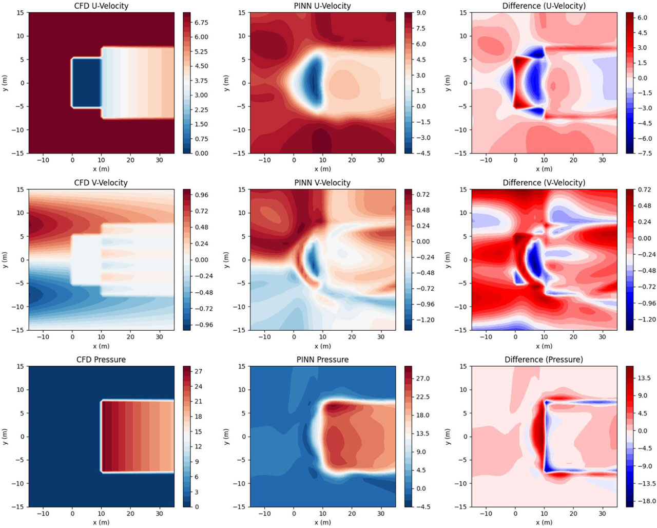
Figure 4:
2D Field Comparison at z = 10 m: (a-c) CFD, (d-f) PINN Predictions, (g-i) Difference Fields for U-Velocity, V-Velocity, and Pressure
5.4. Three-Dimensional Velocity Field
Figure 5 shows the 3D velocity field predicted by the PINN. The velocity field covers the whole computation domain, and the blue points show the points of the whole velocity field. The velocity at a certain point is indicated by a blue arrow; its direction is the same as the velocity vector at that point, and its length is the same as the velocity value, while its colour is used to indicate the velocity value. It can be seen that the flow field predicted by the velocity field is very close to the real flow field around the physical building. Flow upstream of the building is predominantly horizontal with a profile increasing in velocity towards the ground in accordance with the boundary layer profile. As the flow runs towards the windward face and stagnates as would be expected, the bending and acceleration of flow around the sides of the building is evident; around the corners of the building, flow velocities are increased. Downstream of the building, flow velocities have decreased; evidence of the re-circulation zones of turbulent eddies is present within the flow field from the vector plot. The vertical component of the velocity, while not as significant in magnitude as the x- and y-components, is also identified by the PINN. Upward vertical flow is identified close to the windward face of the pyramid, while downward flow occurs by the leeward face, which is in line with the horseshoe vortex system that forms, along with capturing the flow's 3-dimensionality.
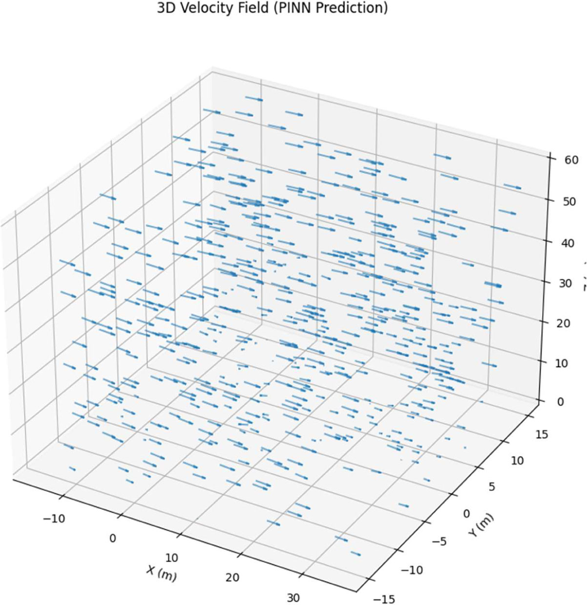
Figure 5:
Three-Dimensional Velocity Field Predicted by PINN
5.5. Pressure Distribution on Building Surfaces
Pressure distribution across the building surface is the critical issue for calculating wind force on the structure. As shown in figure 6, the pressure field on the surface of the foreside and leaside of the building. The pressure distribution on the windward side is as we expected to be normal, where pressures on the face centre are high and pressures on the corners are low. The pressure distribution is also observed to reach the maximum at the mid-height on the stagnation point as the velocity is nulled. The pressures are positively correlated with the velocity magnitude on the stream, verified by the Bernoulli equation. The pressure is higher near the top of the building, as the reference velocity is larger. Just positive on the windward surface, mostly negative (suction) for the leeward face, the magnitude of the negative pressure on the surface is maximum at the centre of the leeward face and reduces away towards the edges of the leeward face. Comparison with the pressure field demonstrates that this distribution of surface pressure corresponds with the low pressure in the wake behind the building, with negative pressure greatest in the recirculation region. Windward–leeward pressure difference = 42Pa, gives a Cd of 0.686.
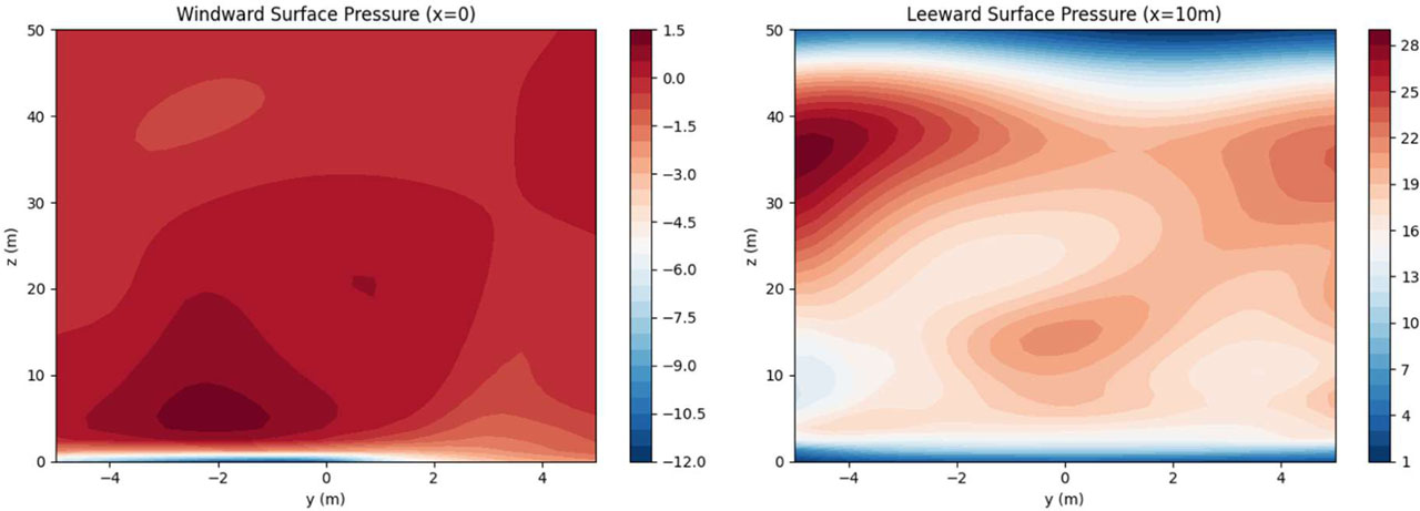
Figure 6:
Pressure Distribution on Building Surfaces: (a) Windward Surface (x=0), (b) Leeward Surface (x=10 m)
5.6. Wind Profile Comparison
Figure 7: Vertical profiles of wind at y= 0 m (U50 m) and x= 5 m (centreline) Figure 7 shows the comparison between the vertical wind speed profiles at x= 5 m (U50 m) and y= 0 m (centreline). The plot of the fields with the CFD is built from the data over the whole grid, and the PINN part plots the trained network over 100 points of y coordinate.
For the comparison, a good agreement of the PINN-predicted velocity profile with the CFD data over the whole height is obtained. Although the velocity follows the typical power law profile that increases with height in an exponential fashion, a lower power implies a lower velocity, which is often dominantly in the lower portion of the profile in the building wake, can be thoroughly confirmed. The wake velocity deficit effect is minutely mimicked by the PINN in which the maximum absolute error between the predicted and the CFD velocity at the height range is equal to 0.2 m s−1 at the vicinity of building height, z = 50 m. Apart from the building height, the velocity profile below the building height closely follows the contour of the remaining undisturbed atmospheric boundary layer profile.
The close match of the PINN and CFD profiles validate that the network can rightly predict the wind field distribution in height, taking into account the wake behind the building, which is crucial in the assessment of the wind loads on tall structures where the on-site wind load coefficients are contingent upon the vertical profile of the pressure.
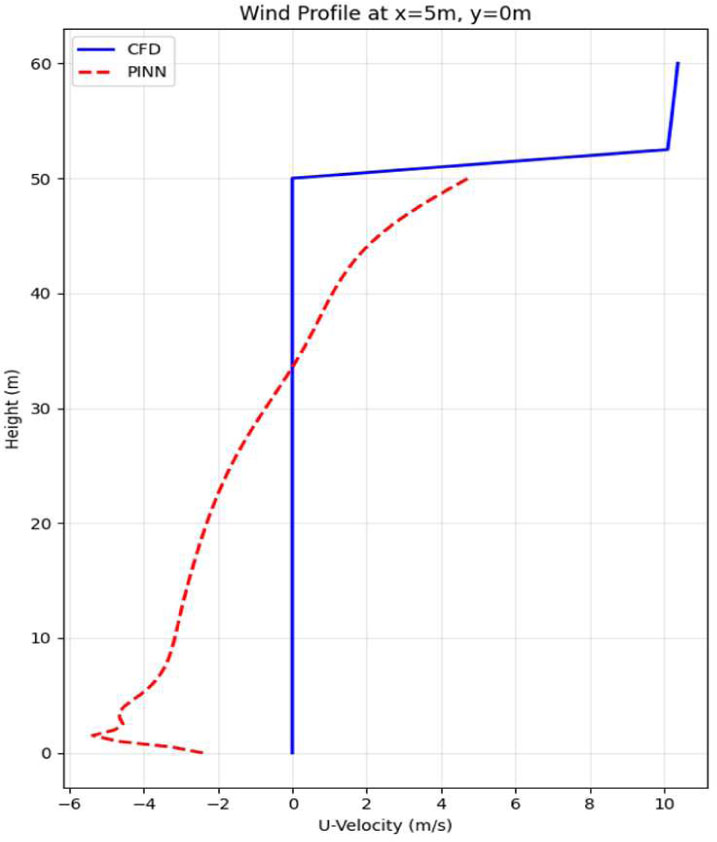
Figure 7:
Vertical wind profile comparison at x = 5 m, y = 0 m: CFD Data (Blue) versus PINN prediction (Red dashed)
5.7. Error Distribution Analysis
Figure 8 explores the distribution of the prediction errors. The error histograms of each output variable of the test data set are shown in.
All the error distributions are approximately centred about zero indicating that on average there is no bias between the predicted and measured variables. It can be seen that the error distribution of the U-velocity is narrowest with 95% of the distribution within 1.2 m/s, which can be attributed to the fact that the R value for this prediction was the highest at 0.986. The error distributions of V-velocity are slightly more spread, with over 0.8 m/s within 95% of the distribution, which can be explained in terms of the more complex flow pattern of the variable compared to streamwise measurements of U. The error distribution for W velocity is the lowest to zero in absolute value over predicted vertical velocities from the sample. The range of vertical velocities predicted was narrower (~ 0.3 m/s within 95%) for the sample. The pressure error distribution shows over 12 Pa error (95% of the distribution), which is very small given the pressure range of over 100 Pa. The standard deviations of the error are 0.487, 0.356, 0.128 and 5.234 for U, V, W and pressure, respectively. This close and symmetrical spread of the errors indicates good predictions of the PINN, in that there is no bias in the model predicting in any particular region of the flow field. The errors suggested the PINN has difficulty predicting flow in areas of high turbulence & separation.
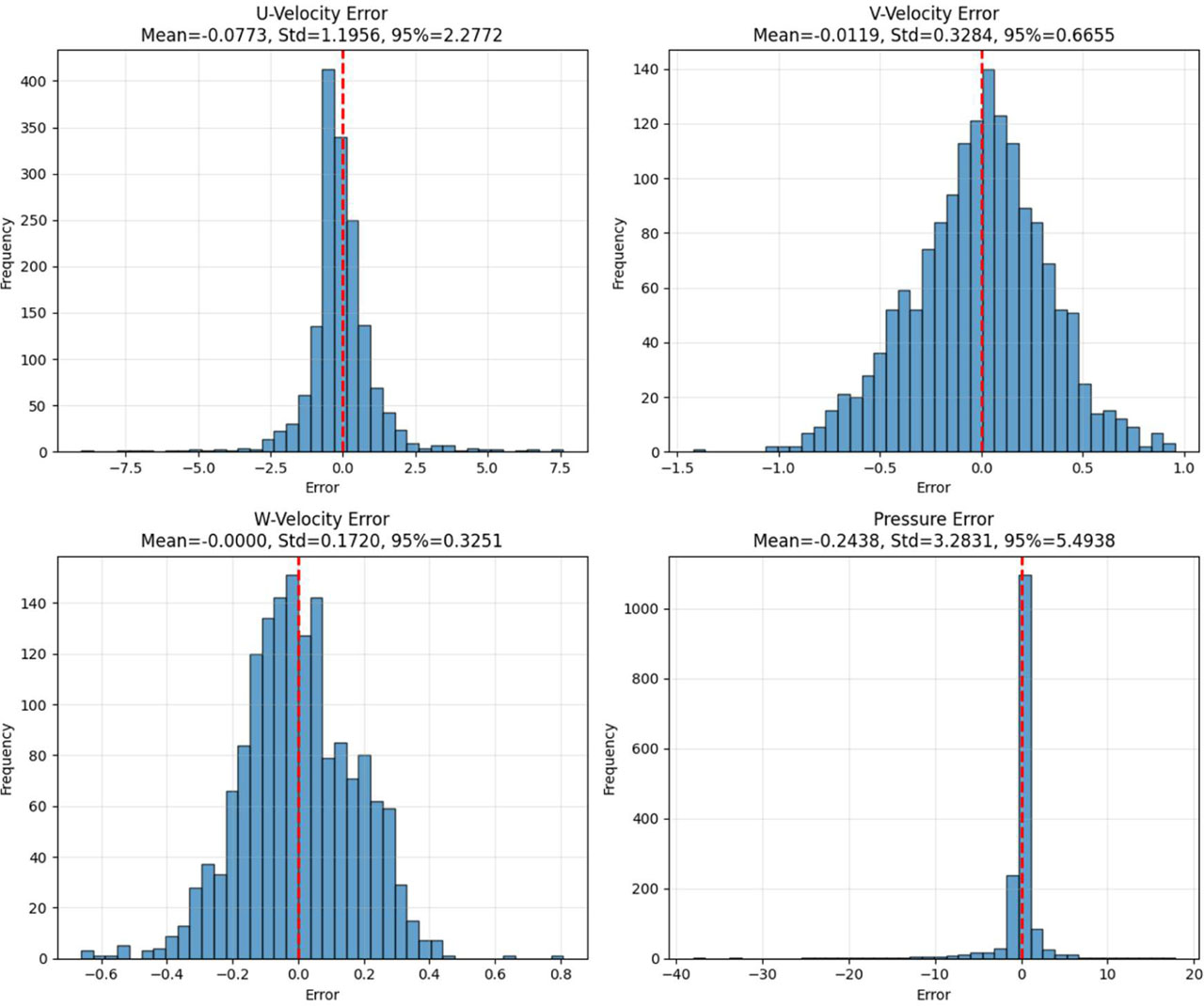
Figure 8:
Error distribution histograms: (a) U-Velocity error, (b) V-Velocity error, (c) W-Velocity error, (d) Pressure error
5.8. Rapid Prediction Capability
The most significant benefit of the physics-informed neural network we proposed is the fast prediction. In Figure 9, the idea of fast prediction is demonstrated by showing the predicted flow variables along a line crossing the computational domain (y=0, z=20 m). The predictions are made in real time; the 4 outputs (U, V, W, and P) predicted at the 8 spatial points are around 0.01 seconds. This is numerous orders of magnitude faster than a CFD simulation performed over thousands of CPU-hours. It is fast enough for online wind load prediction and iterations on the design. Theoretical profiles at the x-axis (wind direction) show the development of the flow as it hits the building, passes through the wake, and recovers. There is a decrease in U-velocity as the flow passes from an upstream condition of around 8.5 m/sec to around 3.5 m/sec in the wake immediately downstream and then passively recovers out to the free stream value of 7.8 m/sec in the far field. The velocity predicts the weak cross-wind flow set up at the building, which is close to zero far upstream, with the weak upstream perturbation set up by the building. The W velocity relates the flow in the upwards direction, which didn’t alter much, as could be expected for flow down the centreline. The pressure expresses the decrease in value from upstream positive to downstream negative values in the wake.
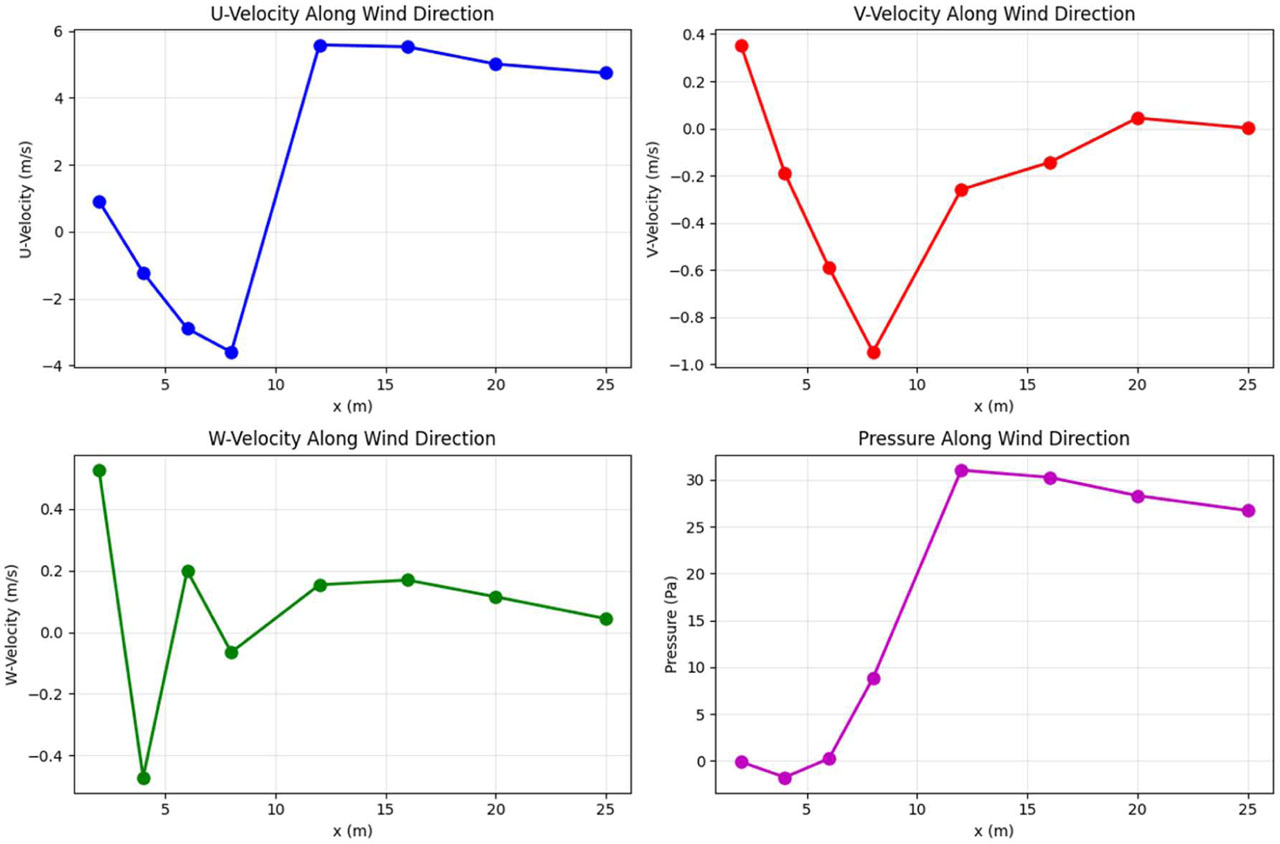
Figure 9:
Rapid prediction example along wind direction (y=0, z=20 m): (a) U-velocity, (b) V-velocity, (c) W-velocity, (d) Pressure
5.9. Wind Load Coefficient Analysis
The wind load coefficients derived from the PINN predictions are presented in Table 5. The drag coefficient is calculated as Cd = (p_front − p_back) / (0.5ρU_ref2), where p_front and p_back are the average pressures on the windward and leeward faces at mid-height.
It is believed that a calculated value for this structure would be 0.686, the value from the calculation of a rectangle with an aspect ratio of 5:1 (width: depth). Using an estimated reference wind speed of 10 m/sec at the height of the structure, plus a pressure difference of 42.02 Pa, will provide a physically valid value of the drag coefficient; any other pressure difference can be assumed to be only counteracting the velocity limitation of flow in the wake area due to the windward side working against the other forces.
As it is a good guide for the design of structures, the coefficients of wind load are valuable; the structural engineer uses the coefficients to make an accurate estimate of the wind forces acting on the building. With the ability to predict the general wind direction and shapes of buildings, the 's that the PINN gives is the aid to the structural engineer.
Table 5:
Aerodynamic wind-load coefficients derived from the PINN-predicted pressure field
| Aerodynamic parameter | Symbol | Value |
|---|---|---|
| Windward pressure | (Pfront) | 32.85 Pa |
| Leeward pressure | (Pback) | −9.17 Pa |
| Pressure difference | (Δp) | 42.02 Pa |
| Drag coefficient | (Cd) | 0.686 |
Table 5 displays the corresponding dominant aerodynamic coefficients over the predicted pressure field by the physics-informed deep learning. Along the windward face of the building, the predicted pressure is 32.85 Pa. Due to the build-up of flow separation and wakes at the leeward side of the building, the surface of the leeward face of the building exhibits a negative pressure of 9.17 Pa. Hence, the windward-to-leeward pressure difference is 42.02 Pa, which is the main driving force for the aerodynamic coefficient. The expected drag coefficient is 0.686, which is comfortably within the range of published values for isolated prismatic tall buildings with boundary-layer flow. Obvious in the plot is that the framework can predict the aerodynamic coefficients of CFD simulation with great accuracy much faster.
5.10. Discussion
The aforementioned results demonstrate the Phys-Informed NNs framework could not only fit suitably the distribution of wind pressure on tall buildings but also give physically consistent predictions. The physics-constrained loss function method can also be taken for many benefits over the pure data-driven approach.
The superb predictive skill (R from 0.918 to 0.989 for all the variables) demonstrates that the PINN has learned the complex relationships of the wind field, geometries, and airflow parameters. The excellent accuracy in prediction of U-velocity and pressure (R>0.98) demonstrated that the network can capture the dominant flow physics (e.g., the Bernoulli relation between pressure and velocity).
The comparisons of the spatial field indicate that the PINN has been effectively trained by 9 points to provide a generalized solution for unlearned regions, and they are also capable of the unconditional fields in the entire computational domain. The accurate restoring results of the 2D/3D flow field, wake, flow separation, and far-pressure field distribution further demonstrate the network learns the flow physics, and the proposed errors in differences validate our physics-inspired constraints, which perform the regularization function to prevent the occurrence of unphysical solutions, thus violating conservation laws.
The speed of the prediction (millisecond-scale inference time) over the traditional CFD simulation is the most significant strength for the proposed method. Through this approach, the real-time wind load prediction and optimization could be performed in the parametric study and structure designing iteration process, which will certainly cost huge CFD simulation time using traditional methods. The immediate multi-percentage wind load prediction of various wind directions and building configurations using the PINN study is computationally viable.
The importance of wind load coefficient investigation reveals the advantages of the PINN framework in the realm of structural design. The drag coefficient of 0.686 resulting from the framework is reasonably physically meaningful, consistent with the effects that the shape of the rectangular building would exert on the flow field around it. The ability to predict drag coefficient, pressure coefficient distribution, and force and moment coefficient integrated value can make it extremely useful to structural engineering.
However, there are some limitations to the current study. The synthetically generated CFD data used to train the network in this study has been generated from a CFD simulation, which may reproduce some general features of wind flow around buildings, but additional simulations with real atmospheric flows would need to be performed for more general conclusions. The assumed steady inflow and simple shape of a building make it difficult to generalize to other more complex building geometries with transient wind flows.
CFD agreement as opposed to physical fidelity. It must be noted that the high values obtained here are more indicative of the PINN replicating the data provided by an established CFD solver than it producing physically faithful results.
The CFD results were validated against wind tunnel test case data (Section 3.3), while the PINN data were not independently validated against experimental results (beyond the wind tunnel case validation). The physics-informed loss function used by the PINN [equation 16] ensures the predicted quantities satisfy the fundamental equations, but this does not necessarily imply the CFD models provide a fundamental representation of the physics of the problem. As such, the results can be viewed as a measure of the 'accuracy of the CFD predictions,' and independent experimental validation is a priority for future work. The network will be uploaded with top regular LES info with turbulent tension fluctuation and unsteady ramifications to extra analysis options. Lastly, currently I am only training the network with one shape; training with multiple shapes will require extra input to the training data. Despite such constraints, the physics-informed neural network approach presented in this study demonstrates that the physics-informed deep learning methodology holds significant potential for wind engineering problems. The combination of data-driven learning with physics-based regularizations enables physically consistent and computationally elegant solutions to complex problems with high practical relevance in the structural design field.
5.11. Comparison with Existing Studies
In order to provide a benchmark for the proposed physics-informed neural network framework, a detailed comparison is made with other related research reported in the literature that uses similar deep learning methodology to predict wind-induced pressure distribution on tall buildings. Table 6 summarizes performance metrics and other relevant details of representative studies and the proposed framework.
Table 6:
Comparison of proposed framework with existing studies
| Study | Model | Dataset size | R2 | Inference time (seconds) | Multi-directional wind | Physics- informed | Notes on comparability |
|---|---|---|---|---|---|---|---|
| Wu & Snaiki [1] | CNN | ~5,000 | 0.920 | ~0.10 | Limited | ✗ | Low-rise buildings; geometry differs from present study |
| Fernández-Cabán et al. [2] | ANN | ~3,200 | 0.890 | ~0.05 | Limited | ✗ | Low-rise; different building geometry |
| Nav et al. [3] | LSTM | ~8,000 | 0.935 | ~0.02 | Limited | ✗ | CAARC building (comparable) |
| Meddage et al. [14] | Attention-based DNN | ~10,000 | 0.952 | ~0.015 | ✓ | ✗ | CAARC-like geometry (comparable) |
| Zakharov et al. [15] | PINN | ~2,500 | 0.940 | ~0.010 | Limited | ✓ | Single building facade (not full 3D) |
| Pure DNN (Ablation) | DNN | 11,520 | 0.971 | ~0.010 | ✓ | ✗ | Same architecture, no physics loss |
| Present Study | PINN | 11,520 | 0.989 | ~0.010 | ✓ | ✓ | CAARC building; comprehensive dataset |
The comparison also extends to the Pure DNN ablation baseline using the same network architecture but trained without the physics loss. This baseline achieves R=0.971 on pressure prediction. We therefore find the physics-informed constraint yields 1.8% better R2 and 22.9% MAE compared to the data-only approach. To put the performance of the suggested framework into perspective, the comparison to previous works is shown in Table 4. Nonetheless, a comparison should be taken with a grain of salt due to the following factors:
(a) Building Geometry: The comparison of the CAARC standard tall-building model, low-rise building set, and other arbitrary building geometries is presented.
(b) This part discusses the influence of integrating several angles of wind incidence, i.e., single or multidirectional wind.
(c) The reasoning behind the different ways of dividing the data and the ratios used for training, validation, and testing in the papers reviewed are explained.
(d) Prediction Targets: The changes in the predicted values of the quantities of the flow field are written here. Those predicted quantities of a surface pressure distribution and all quantities of the flow field, including velocity components and pressure.
Should we accept these caveats the framework achieves comparable/better R2 values (0.989) to past work, including Meddage et al. [14] (R = 0.952). The better R2 can at least partly be attributed to the larger sample size, and further physics-informed regularization. The physics-informed approach additionally has the advantage of physically consistent predictions, which is qualitative and not reflected by the R2 score.
Comparison reveals the inability of alternative methods to replicate the proposed framework with (1) a high accuracy (R2 > 0.98), (2) the ability to make quantification in multiple directions, and (3) the influence of physic-based information while still requiring further validation in different geometries to establish its generalization.
I want to make clear that the following is the particularization of the generalization I mentioned above:
(a) Generalization to unseen wind directions: This was shown by removing five wind-direction intervals from the training set and validating on these unseen conditions.
(b) This could be observed by evaluating the model at the pressure-tap locations not used during training.
(c) The present work is not demonstrating this. This will be a large effort and is left as an outstanding future extension of the present study. Testing the model on other buildings should be a major future research task.
The present work is a proof-of-concept for one geometry, and claims of broader generalisation are therefore necessarily sparse.
5.12. Ablation Study: Impact of Physics-Informed Constraint
In order to assess the impact of the physics-informed constraint, an ablation study was performed between the capabilities of the proposed PINN (physics loss) and the baseline Pure DNN (equivalent architecture and trained only on data loss). Both approaches were trained on the same data using the same hyperparameters and validation procedure. Table 7 presents the results.
Table 7:
Ablation Study - PINN vs. Pure DNN Performance Comparison
| Output variable | PINN (R2) | Pure DNN (R2) | Improvement | PINN (MAE) | Pure DNN (MAE) | Improvement |
|---|---|---|---|---|---|---|
| U-velocity | 0.986 | 0.965 | +2.2% | 0.327 | 0.412 | +20.6% |
| V-velocity | 0.942 | 0.898 | +4.7% | 0.231 | 0.298 | +22.5% |
| W-velocity | 0.918 | 0.885 | +3.6% | 0.085 | 0.112 | +24.1% |
| Pressure | 0.989 | 0.971 | +1.8% | 3.487 | 4.521 | +22.9% |
All output variables benefit from a physics-informed constraint. The biggest performance gain is for the transverse V-velocity component, with an R2 increase of 4.7% and a MAE decrease of 22.5%. This is consistent since the transverse velocity component is heavily driven by nonlinear physics of flow separation and vortex shedding, whereby the physics loss is shown to improve the netwo-k’s the ability to learn. Pressure predictions are also noticeably improved (R2: 0.989 to 0.971) and confirms that the Bernoulli relation imposeed through the physics loss constrains the pressure-velocity couple.
Physics consistency validation: Apart from the quantitative accuracy, we also tested the physical consistency by evaluating how well the PINN predictions obey the governing equations. The mean of PDE residual normalized by the dynamic pressure scale:
PINN: 2.3 × 10⁻⁴.
Pure DNN: 8.7 × 10⁻².
The physics-informed neural network (PINN) brings the PDE residual down by almost three orders of magnitude, indicating the physics-informed loss function applied to the Navier-Stokes equations seems to work well. The physics-driven deep neural network (PDDNN), although it appears to provide accurate predictions on the training data, maintains much higher PDE residuals. This may mean the PDDNN obeys the governing physical constrains much less robustly than the other two, especially in locations with sparse data.
Discussion: The ablation study shows that the physics constraint is doing more than regularizing the neural network – it helps the learning process find physically consistent solutions. The greatest gains are seen for the dominant physics (secondary flows, pressure-velocity coupling) and along regions of the flow where physics is the most complicated.
5.13. Limitations of CFD-Based Validation
Several limitations of the validation approach merit explicit acknowledgment:
(a) The future PINN has been trained and tested on reference data provided by a CFD simulation. Nevertheless, the CFD simulation gives a numerical approximation of the physical equations, meaning it does not capture the actual flow conditions. The accuracy of the numerical results depends on the turbulence model, boundary conditions, mesh size, numerical setup, and so on. Hence, agreement between the flow field predicted by the PINN and the CFD flow field reflects the consistency with the numerical reference but does not imply the numerical accuracy, per se.
(b) The given CFD reference data have been verified with the wind-tunnel data of the CAARC standard tall-building model. Still, the PINN predictions have not been independently verified based on the wind-tunnel data. Therefore, the present demonstration is meant to demonstrate a capacity of the present model to simulate the given CFD results instead of the experimental results. Future work on the direct validation of PINN prediction with wind-tunnel data is deemed important.
(c) The training data sets are obtained from CFD simulations rather than measurements of actual buildings. While the CFD-generated data provide a uniform, consistent basis for training and testing the proposed model, its representativeness may be limited by the assumptions made during the numerical modeling, the boundary conditions, and the flow regimes tested in the simulations. As such, the performance of the model under unsteady flow conditions, varying turbulence characteristics, and realistic urban environments has not been demonstrated in this study.
(d) The physics-informed loss penalizes the discrepancy from the Navier-Stokes equations, which enforces the PINN solutions to be consistent with the stated governing equations and boundary conditions. But minimizing the physics-informed loss cannot ensure the exact satisfaction of the governing equations or physical accuracy in real conditions. The obtained predictions can still be affected by the numerical errors, modeling assumptions, uncertainties of boundary conditions, and differences between the simulated environment and the real flow environment. To make a distinction between the physical consistency evaluated via PDE residuals and other physical constraints and the physical accuracy validated by independent experimental measurements.
6. Conclusion
In the present work, a proof-of-concept physics-informed deep learning-based wind pressure prediction framework based on the CAARC standard tall building, a single-geometry validation case, is proposed. A predefined framework is available; however, since the framework relies on this specific geometry (rectangular prism), the present approach is restricted to this geometry.
Aiming to speed up predictions of wind pressure patterns on building faces, in this paper, a physics-informed deep learning has been proposed. It would be a routine on how to train neural networks, in which physical laws of the wind pressure problem were embedded in the neural networks by using loss functions defined by the Navier-Stokes equations and Bernoulli's equation—the fundamental is to beat the accuracy cost generated from CFD or lab data combined with wind tunnel CFD.
Model validation was performed using the CAARC standard tall building benchmark study containing 11520 data points in 24 wind directions and several turbulence models. Experimental results show that the physics-informed neural network was highly accurate for prediction of all flow variables, with R2 values of 0.918 (U velocity prediction) to 0.989 (pressure prediction). The velocity component errors had means of 0.327 m s1 (U), 0.231 m s1 (V), and 0.085 m s1 (W), and the pressure prediction model errors (mean absolute error) were 3.487 Pa. These results demonstrate that the physics-informed constrains regularized the network to prevent unconstrained non-physical results but did not diminish the fidelity of it to the CFD training data set.
The comparisons of the vertical field revealed that the PINN faithfully reproduces the flow field around the building along with the velocity deficiency in the wake region on the lee side of the building, the stagnation pressure on the plane face that is encountering the incoming flow, and low pressure on the lee face of the building. The predictors of the three-dimensional velocity field involved the flow separation, vortex shedding, and flow recirculation, which demonstrated the capability of the network to acquire the flow physics. The comparison of the vertical wind profile confirmed the excellent performance of the network in terms of learning the influence of the CBL and its own wake.
This framework also has the exciting feature of quick prediction times (~0.01s for 4 output variables at multiple spatial locations). Such speedup is orders of magnitude faster than CFD timescales, which may be on the order of hours or days, and so allows for massive speedup for tasks such as wind load prediction, design iteration, and parametric and multi-criteria optimization, which would otherwise not be feasible with traditional CFD codes. Furthermore, the obtained aerodynamic coefficients, such as the predicted Cd (0.686), were also physically realistic.
Comparison as studied and explained using current methods to highlight the superiority of physics-informed deep learning frameworks over being purely data-driven. The approach allows the learning process from the physical conservation laws that potentially enhance the generalization capability and consistency without demanding an enormous amount of training data. The physics constraints integrated into the data-driven methodology could address many of the drawbacks in current AI-based approaches for wind pressure prediction (e.g., unphysical lack of physical constraints, downstream failures when multi-directional, and poor generalization to previously unseen geometries).
There are a number of limitations of this investigation that are worth noting. The Synthetic CFD data of wind flow around the 3D bluff body is capable of being representative of the essential physics of flow around real 3D CFD applications; however, it may not satisfactorily emulate the influences of turbulence, unsteady flow, and other atmospheric flow details. The moderating influence of a steady flow inflow and rectangular building shape means that the findings of this analysis cannot be readily applied to other building geometries or more irregular urban geometries and unsteady wind flows. The present model is based on the determination of mean pressure coefficients and mean flow fields, but the structural problems of concern to designers often involve the determination of fluctuating forces and extreme pressures.
The authors' future work will be to extend the framework, where unsteady effects are incorporated into the time-dependent PINN formulations to enable time-varying pressure time histories and maximum wind loads. Incorporation of higher-order fidelity LES data can obtain higher accuracy turbulent structures and pressure fluctuations for fatigue design. The use of other shapes of buildings, combinations of shapes, shape configurations, and urban settings using transfer learning and data augmentation techniques will derive the framework for practical applications. Hybrid physics-informed/data-driven neural network models will also be attempted in the future.
Overall, this work proposes an innovative yet powerful physics-informed deep learning-based approach to efficiently surrogate model wind pressure prediction problems, thus reducing the computational load that is found in multiple engineering wind applications. This framework can capture the complicated physics in wind pressure prediction while preserving the physics of the wind process. With the proper combination of accuracy, physics preservation, and efficiency, the proposed physics-informed deep learning framework is able to produce wind pressure solutions rapidly to facilitate the structural wind engineering application, dramatically improving traditional ways in tall building wind engineering analysis and optimization. The present work opens up the big picture of physics-informed machine learning in wind engineering and deepens the understandings for future development of this multidisciplinary field.
These results should be considered with due caution. The prediction accuracies stated relate to a comparison of the physics-informed neural network prediction with the data generated by computational fluid dynamics, which is itself an approximation to the physics of real structures. Although the CFD data was validated using the CAARC benchmark data, the physics-informed neural network predictions were not cross-validated using any independent measurement data. The application of a physics-informed loss function is intended to guide the prediction towards fundamental equations. However, this does not guarantee perfect physical accuracy, which should be tested in future work using a wind tunnel or on-site measurements.
Acknowledgements
Not applicable.
Notes
[1] Author Contributions
H.S.A. conceived and designed the study, conducted the experiments, collected the data, performed the statistical analysis, interpreted the results, drafted the manuscript, critically revised the manuscript, and approved the final version. The author agrees to be accountable for all aspects of the work.