

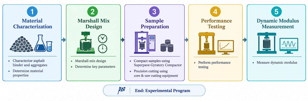
Figure 1:
Experimental program to acquire data for predicting dynamic modulus
Table 1:
Key properties of aggregates
| Aggregate Property | Reference Standard | Average Value [%] | Value Range [%] |
|---|---|---|---|
| Soundness | AASHTO T104 | 3 | ≤12 |
| Sand Equivalent Value | AASHTO T 176 | 72 | ≥ 45 |
| Elongation Ratio | ASTM D 4791 | 7 | ≤ 10 |
| Flakiness Ratio | ASTM D 4791 | 5 | ≤ 10 |
| Los Angeles Abrasion | AASHTO T96 | 26 | ≤ 30 |
Table 2:
Gradation blend details
| Gradation Blend | Sieve Size [mm]/Percent Passing [%] | ||||||||
|---|---|---|---|---|---|---|---|---|---|
| 37.5 | 25.0 | 19.0 | 12.5 | 9.5 | 4.75 | 2.36 | 0.30 | 0.075 | |
| GB-1 | - | - | - | 82.5 | 68.7 | 49.3 | 30.8 | 10.5 | 5.2 |
| GB-2 | - | - | 99.9 | 79.5 | 69.4 | 48.7 | 35.3 | 11.8 | 5.2 |
| GB-3 | - | - | 99.7 | 84.5 | 63.4 | 46.0 | 30.5 | 10.3 | 5.0 |
| GB-4 | - | - | - | 80.0 | 67.0 | 48.0 | 33.0 | 11.0 | 4.7 |
| GB-5 | - | 82.6 | 69.7 | 59.2 | 52.2 | 41.6 | 24.5 | 9.4 | 5.0 |
| GB-6 | - | 85.4 | 71.0 | 59.9 | 53.4 | 35.5 | 26.4 | 10.8 | 4.7 |
| GB-7 | 98.8 | 82.7 | 67.4 | 56.2 | 43.5 | 35.0 | 25.1 | 7.6 | 4.2 |
| GB-8 | - | - | 95.0 | 76.0 | 63.0 | 42.5 | 29.0 | 8.5 | 5.0 |
| GB-9 | - | - | - | 82.0 | 70.0 | 50.0 | 30.0 | 10.0 | 5.0 |
| GB-10 | - | - | - | 94.0 | 87.0 | 65.0 | 37.0 | 9.0 | 5.0 |
| GB-11 | - | - | - | 95.0 | 82.0 | 59.0 | 43.0 | 13.0 | 6.0 |
| GB-12 | 95.0 | 77.0 | 65.5 | 52.5 | 44.0 | 31.5 | 22.5 | 7.0 | 4.5 |
| G-13 | - | 82.5 | 72.5 | 62.5 | 52.5 | 37.5 | 25.0 | 10.0 | 4.5 |
| GB-14 | - | 95.0 | 85.0 | 60.0 | 47.0 | 30.0 | 20.0 | 8.0 | 4.0 |
| GB-15 | - | 95.0 | 83.0 | 70.0 | 63.0 | 52.0 | 39.0 | 14.0 | 5.5 |
| GB-16 | - | - | 95.0 | 83.0 | 65.0 | 46.0 | 30.0 | 9.0 | 5.0 |
Table 3:
Key properties of bitumen
| Bitumen Property | Reference Standard | ARL 40/50 | ARL 80/100 | ARL 60/70 | NRL 60/70 |
|---|---|---|---|---|---|
| Penetration Value [0.1 mm] | AASHTO T49 | 43 | 84 | 66 | 64 |
| Softening Point [°C] | AASHTO T53 | 52 | 46 | 48.8 | 49.2 |
| Flash and Fire Points [°C] | AASHTO T48 | 335 & 359 | 233 & 275 | 304 & 334 | 310 & 343 |
| Viscosity at 135°C [ Pa·s] | AASHTO T316 | 0.486 | 0.226 | 0.241 | 0.292 |
Table 4:
Summary of mix design parameters using the Marshall method
| Bitumen Source/Type | Gradation Blend | Air Voids [%] | Optimum Binder Content [%] | Voids in Mineral Aggregate [%] | Voids Filled with Asphalt [%] | Stability [Kg] | Flow [mm] |
|---|---|---|---|---|---|---|---|
| ARL 40/50 | G-8 | 4.0 | 3.9 | 13.09 | 69.44 | 1198 | 2.29 |
| G-10 | 4.0 | 5.5 | 15.22 | 73.71 | 1447 | 2.63 | |
| G-14 | 4.0 | 3.4 | 13.16 | 69.62 | 2243 | 3.40 | |
| G-15 | 4.0 | 4.4 | 13.55 | 70.48 | 3114 | 9.00 | |
| ARL 80/100 | G-8 | 4.0 | 3.7 | 11.32 | 64.66 | 790 | 2.68 |
| G-10 | 4.0 | 4.6 | 15.04 | 73.40 | 934 | 2.58 | |
| G-14 | 4.0 | 3.3 | 11.45 | 65.07 | 2526 | 8.81 | |
| G-15 | 4.0 | 4.3 | 12.30 | 67.50 | 610 | 7.52 | |
| ARL 60/70 | G-3 | 4.0 | 4.2 | 14.20 | 66.50 | 1343 | 3.10 |
| G-4 | 4.0 | 4.2 | 13.40 | 59.50 | 1298 | 2.99 | |
| G-7 | 4.0 | 3.5 | 12.80 | 58.00 | 2632 | 5.02 | |
| G-8 | 4.0 | 4.0 | 12.15 | 66.08 | 1362 | 3.00 | |
| G-9 | 4.0 | 4.1 | 12.95 | 65.16 | 1291 | 3.16 | |
| G-10 | 4.0 | 5.0 | 14.70 | 69.18 | 1424 | 3.38 | |
| G-11 | 4.0 | 4.8 | 14.52 | 67.73 | 1544 | 3.28 | |
| G-12 | 4.0 | 3.3 | 11.38 | 62.19 | 2650 | 4.81 | |
| G-13 | 4.0 | 3.7 | 11.87 | 63.33 | 2905 | 4.66 | |
| G-14 | 4.0 | 3.6 | 12.17 | 61.93 | 2295 | 5.38 | |
| G-15 | 4.0 | 3.9 | 12.40 | 61.33 | 3496 | 4.53 | |
| G-16 | 4.0 | 4.36 | 14.43 | 74.53 | 3235 | 9.12 | |
| NRL 60/70 | G-1 | 4.0 | 4 | 14.8 | 66.9 | 1290 | 2.88 |
| G-2 | 4.0 | 4.4 | 15.3 | 63.5 | 1330 | 3.052 | |
| G-5 | 4.0 | 3.3 | 13.7 | 58.1 | 2890 | 4.302 | |
| G-6 | 4.0 | 3.4 | 13.2 | 59.2 | 2620 | 4.981 |
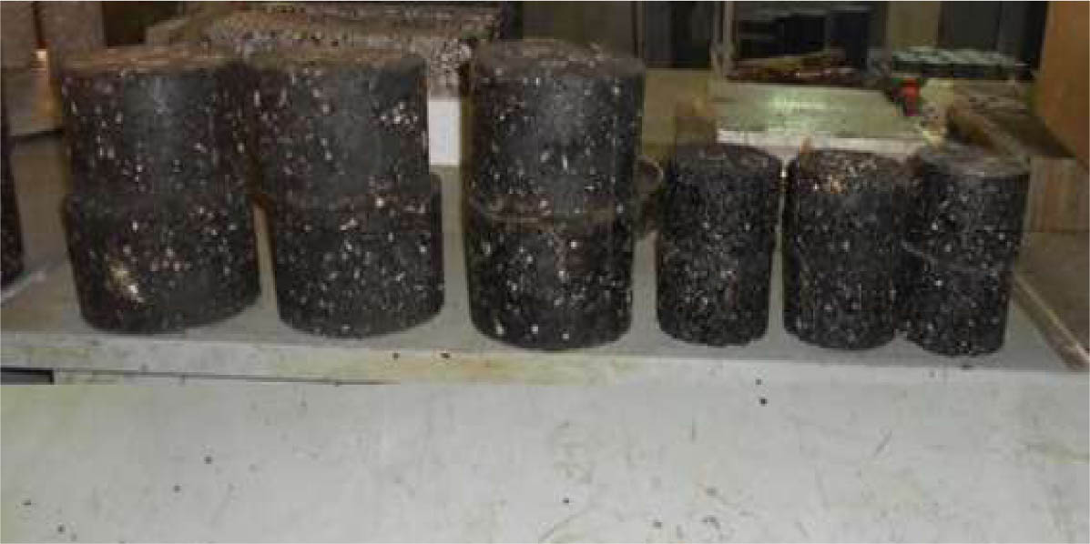
Figure 2:
Representative HMA specimens at different bitumen contents
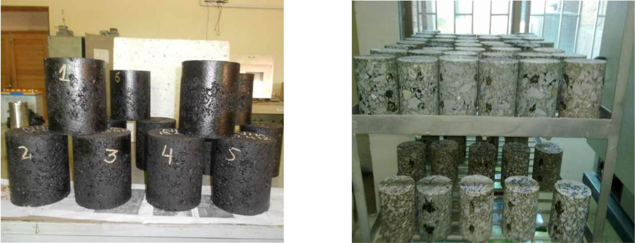
Figure 3:
Core and uncore specimens for dynamic modulus testing
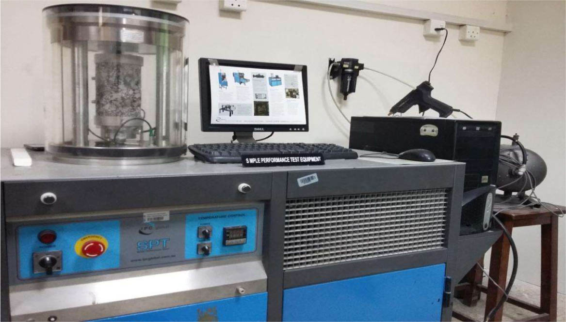
Figure 4:
Conducting SPT on a cored sample
Table 5:
Model configurations and hyperparameters used in the MATLAB Regression Learner application
| Model | MATLAB function | Model specification | Main settings |
|---|---|---|---|
| LR | fitlm | Linear regression | RobustOpts = off |
| ILR | fitlm | Interaction regression | RobustOpts = off |
| FT | fitrtree | Fine regression tree | MinLeafSize = 4; Surrogate = off |
| MT | fitrtree | Medium regression tree | MinLeafSize = 12; Surrogate = off |
| QSVM | fitrsvm | Quadratic polynomial SVM | PolynomialOrder = 2; KernelScale = auto; BoxConstraint = IQR/1.349; Epsilon = IQR/13.49; Standardize = true |
| CSVM | fitrsvm | Cubic polynomial SVM | PolynomialOrder = 3; KernelScale = auto; BoxConstraint = IQR/1.349; Epsilon = IQR/13.49; Standardize = true |
| EBT | fitrensemble | LSBoost | 30 learning cycles; LearnRate = 0.1; tree MinLeafSize = 8; variables sampled = all |
| EBagT | fitrensemble | Bagging | 30 learning cycles; tree MinLeafSize = 8; variables sampled = all |
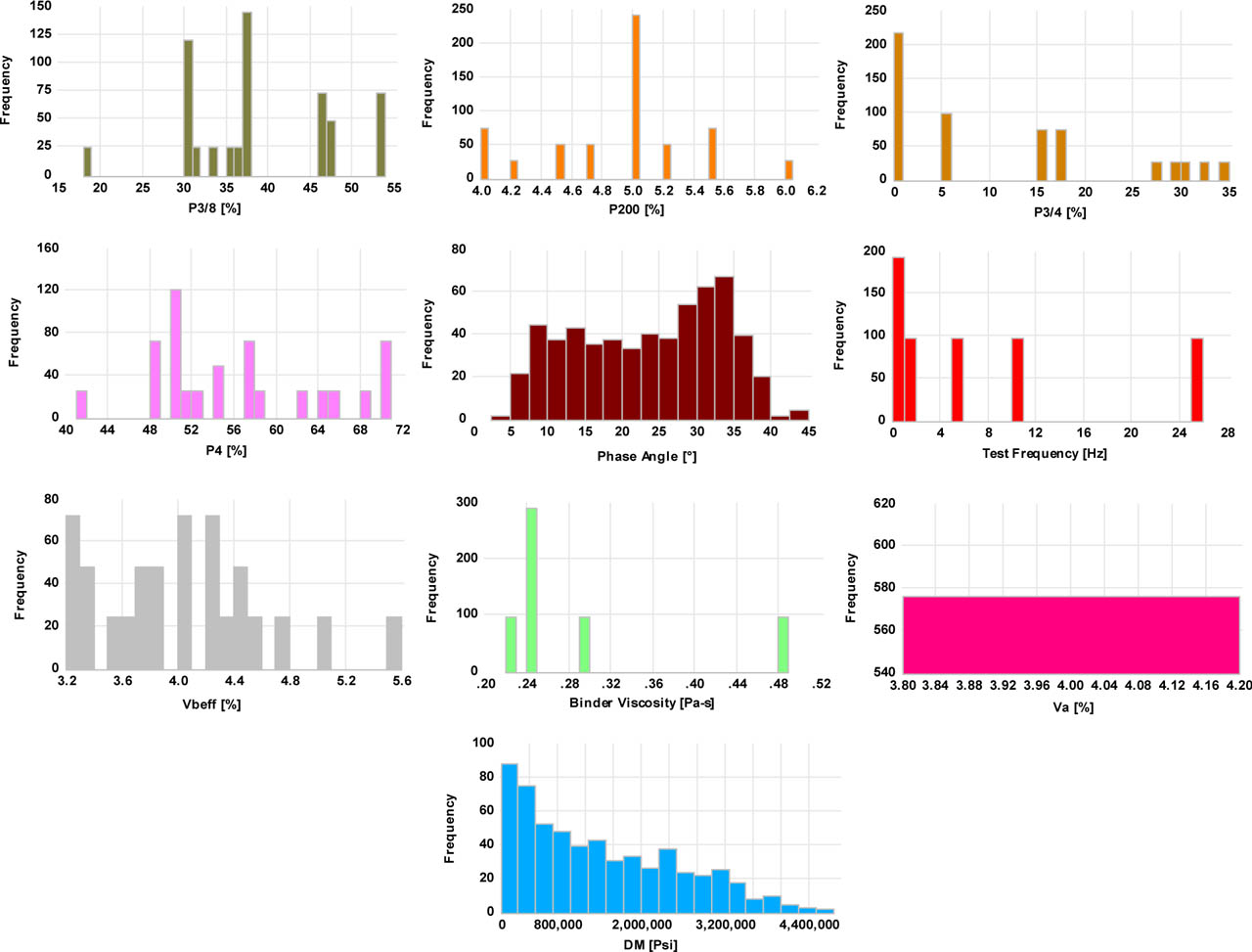
Figure 5:
Histogram matrix showing the frequency distributions of key material and rheological parameters
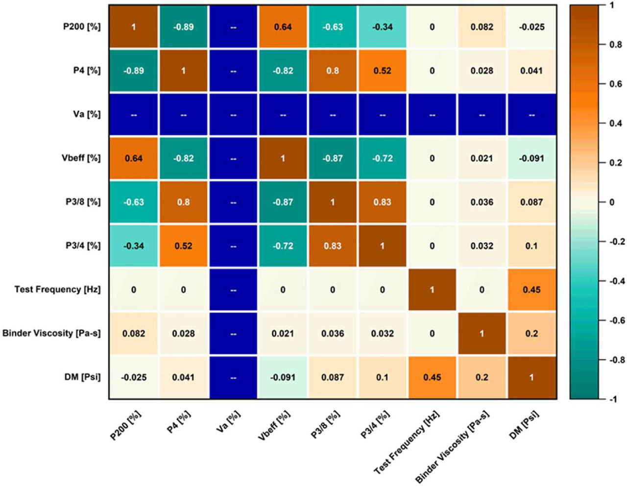
Figure 6:
Spearman Correlation matrix heatmap showing relationships among mixture components
Table 6:
Metric analysis results for all models
| Model | RMSE [psi] (Validation) | MSE [psi2] (Validation) | R2 [-] (Validation) | MAE [psi] (Validation) | MAE [psi] (Test) | MSE [psi2] (Test) | RMSE [psi] (Test) | R2 [-] (Test) |
|---|---|---|---|---|---|---|---|---|
| LR | 3.87 × 10⁵ | 1.50 × 10¹¹ | 0.86 | 3.00 × 10⁵ | 2.93 × 10⁵ | 1.32 × 10¹¹ | 3.64 × 10⁵ | 0.90 |
| ILR | 3.22 × 10⁵ | 1.03 × 10¹¹ | 0.90 | 2.32 × 10⁵ | 2.05 × 10⁵ | 7.78 × 10¹⁰ | 2.78 × 10⁵ | 0.94 |
| FT | 3.97 × 10⁵ | 1.58 × 10¹¹ | 0.85 | 3.11 × 10⁵ | 2.86 × 10⁵ | 1.49 × 10¹¹ | 3.86 × 10⁵ | 0.89 |
| MT | 4.37 × 10⁵ | 1.91 × 10¹¹ | 0.82 | 3.38 × 10⁵ | 2.86 105 | 1.46 × 10¹¹ | 3.82 × 10⁵ | 0.89 |
| QSVM | 2.78 × 10⁵ | 7.73 × 10¹⁰ | 0.93 | 1.96 × 10⁵ | 1.80 × 10⁵ | 6.18 × 10¹⁰ | 2.48 × 10⁵ | 0.95 |
| CSVM | 2.32 × 10⁵ | 5.39 × 10¹⁰ | 0.95 | 1.67 × 10⁵ | 1.51 × 10⁵ | 4.90 × 10¹⁰ | 2.21 × 10⁵ | 0.96 |
| EBT | 3.11 × 10⁵ | 9.67 × 10¹⁰ | 0.91 | 2.40 × 10⁵ | 2.08 × 10⁵ | 7.99 × 10¹⁰ | 2.82 × 10⁵ | 0.94 |
| EBagT | 3.42 × 10⁵ | 1.17 × 10¹¹ | 0.89 | 2.55 × 10⁵ | 2.21 × 10⁵ | 8.73 × 10¹⁰ | 2.95 × 10⁵ | 0.93 |
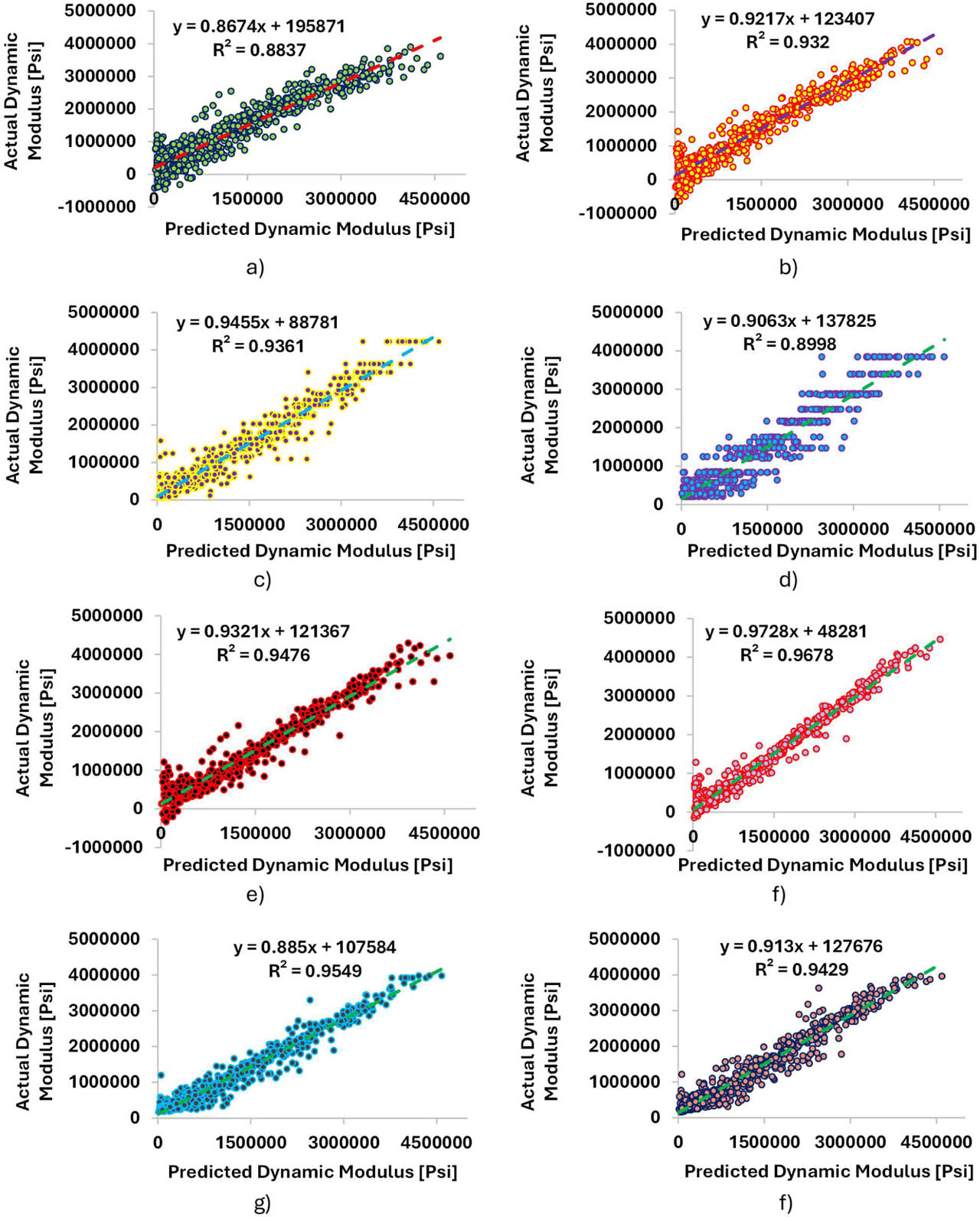
Figure 7:
Actual vs predicted dynamic modulus (Psi) a) LT b) ILT c) FT d) MT e) QSVM f) CSVM g) EBT h) EBagT
Table 7:
Sensitivity Analysis for phase angle
| Model | Phase Angle [-] | No-Phase Angle [-] | Phase Angle RMSE [psi] | No-Phase Angle RMSE [psi] |
|---|---|---|---|---|
| LR | 0.90 | 0.0704 | 3.64 × 10⁵ | 1.03 x 10⁶ |
| ILR | 0.94 | 0.0636 | 2.78 × 10⁵ | 1.03 x 10⁶ |
| FT | 0.89 | −0.2180 | 3.86 × 10⁵ | 1.17 x 10⁶ |
| MT | 0.89 | −0.0855 | 3.82 × 10⁵ | 1.11 x 10⁶ |
| QSVM | 0.95 | −0.0219 | 2.48 × 10⁵ | 1.07 x 10⁶ |
| CSVM | 0.96 | −0.1854 | 2.21 × 10⁵ | 1.16 x 10⁶ |
| EBT | 0.94 | 0.0150 | 2.82 × 10⁵ | 1.05 x 10⁶ |
| EBagT | 0.93 | 0.0262 | 2.95 × 10⁵ | 1.05 x 10⁶ |
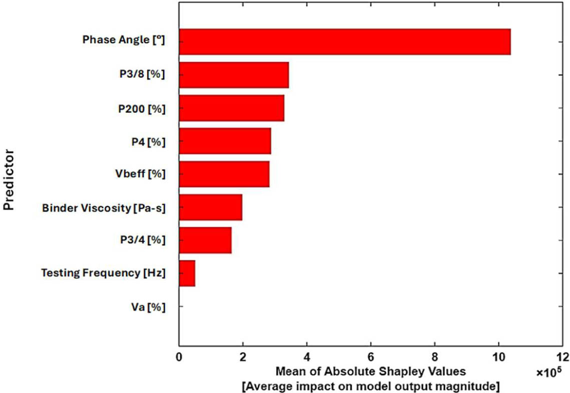
Figure 8:
Shapley feature importance analysis for Model [Cubic SVM]
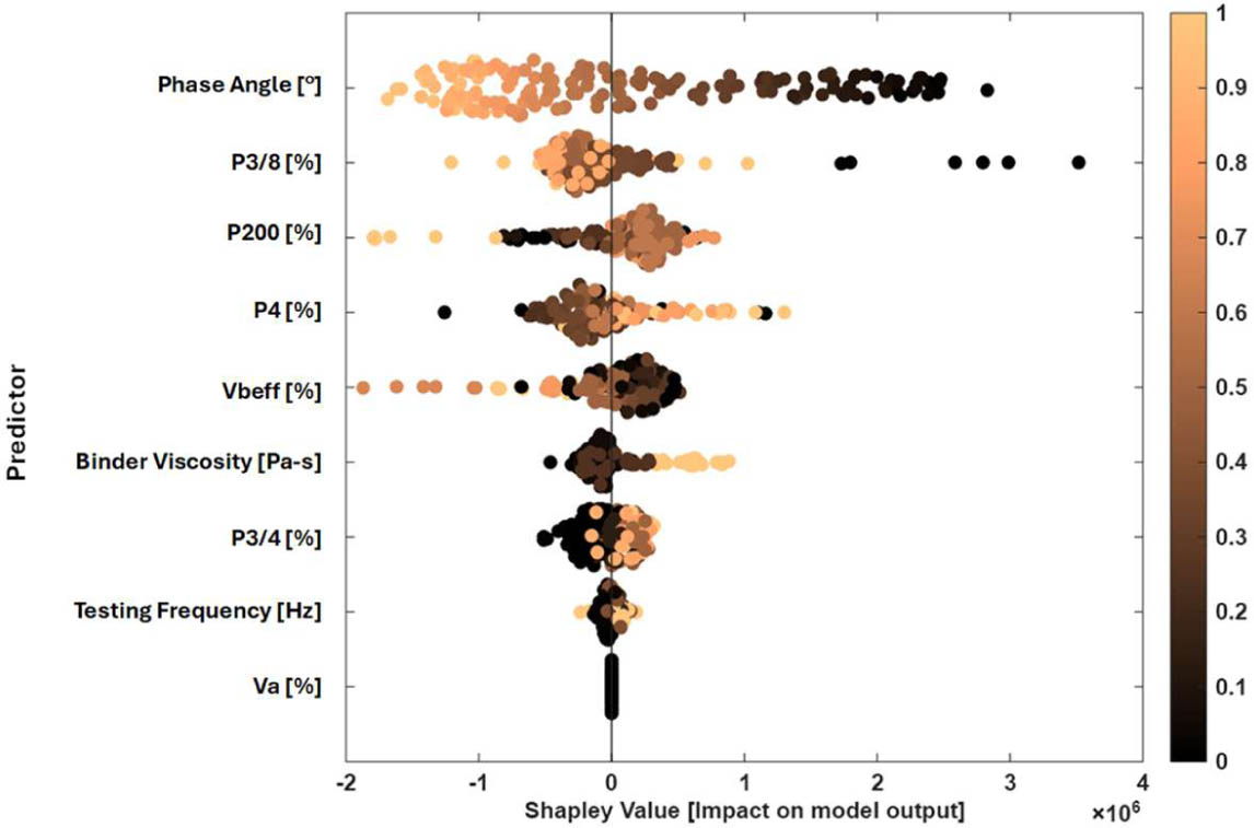
Figure 9:
SHAP summary plot for the Cubic SVM model
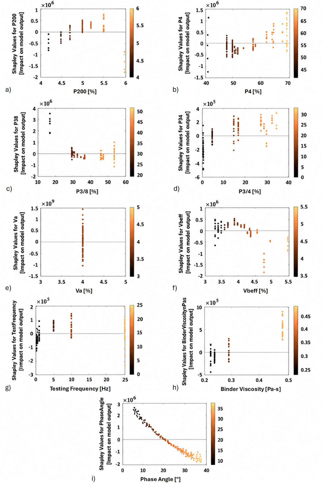
Figure 10:
SHAP dependence plots for the Cubic SVM model