

1. Introduction
Hot Mix Asphalt (HMA) is widely adopted for pavement construction worldwide. Its workability and durability are among the primary reasons for its extensive application in pavements (Han et al., 2021b). It provides resistance against two primary forms of pavement distress, namely rutting and moisture damage. The resistance of HMA against these distresses can be further improved through the use of additives (Al Hawesah et al., 2021). Due to the high energy requirements and other environmental impacts associated with the production of HMA, Warm Mix Asphalt (WMA) and Reclaimed Asphalt Pavement (RAP) have also been introduced as alternative approaches in many applications (Sukhija & Coleri, 2025). However, HMA continues to be extensively employed in pavement design and construction (Bellary & Kadli, 2023), particularly because of its proven performance under diverse traffic and climatic conditions worldwide.
Dynamic Modulus (DM), mathematically represented by |E*|, is a critical mechanical property of HMA that characterizes its response to cyclic loading and reflects both its elastic and viscous behavior under different loading conditions (Belhaj et al., 2024). As a fundamental measure of asphalt mixture stiffness, DM is closely related to the resistance of pavement layers to traffic-induced deformation and is therefore an important input for mechanistic-empirical pavement design. Higher DM values generally indicate greater mixture stiffness, whereas lower values reflect a more compliant response under the corresponding loading conditions. Hence, it is strongly influenced by the viscoelastic behavior of asphalt mixtures (Solatifar, 2020). It can be measured in the laboratory under different temperatures, loading frequencies, and loading conditions (Bi et al., 2021; Junaid et al., 2022). These variations highlight the importance of considering multiple material and testing parameters when characterizing and predicting the DM of HMA mixtures.
In addition to the viscoelastic properties of the asphalt binder, its shear modulus also significantly affects DM (Owais & Moussa, 2024). Binder modifications, such as the addition of polymers, can alter binder stiffness and consequently modify the mechanical response of the asphalt mixture. Other mixture constituents also contribute to DM; for example, the ratio of mineral filler to asphalt binder affects mixture stiffness (Bi et al., 2021). Aggregate characteristics are also important, with the maximum aggregate size generally showing a positive relationship with mixture stiffness (Ghafarpour & Khodaei, 2009). Furthermore, mix-design characteristics, including volumetric properties such as air voids (Va) and binder content, as well as construction methods, can influence the resulting mechanical response (Islam et al., 2019). Environmental conditions, including temperature, moisture, and ageing, can further alter the stiffness and viscoelastic behavior of asphalt mixtures (Yan et al., 2024; Junaid et al., 2024a). The interaction of these materials makes DM a complex property that cannot be adequately characterized using only a limited set of explanatory variables.
DM of asphalt mixtures plays an important role in the design and performance evaluation of road pavements because it provides an indication of mixture stiffness and resistance to traffic-induced deformation (Imoh et al., 2026). Consequently, accurate prediction of DM requires consideration of a wide range of interacting material and mix-design parameters. The current models for predicting DM are largely based on empirical or semi-empirical relationships developed under specific materials, testing conditions, and datasets (Vestena et al., 2021). These models may lack the flexibility required to accommodate variations in materials, mixture characteristics, and construction practices, which are continuously modified to improve the sustainability, performance, and efficiency of pavement construction. Moreover, conventional empirical models generally rely on predefined functional relationships, which may not adequately capture the nonlinear and complex interactions among the factors governing DM. With these innovations, there is a greater need to understand both the predictive relationships and the relative importance of individual parameters affecting the DM of HMA mixtures.
Use of robust Artificial Intelligence (AI) techniques can provide valid tools for a generic design optimization of HMA mixtures. Unlike conventional empirical approaches, AI-based methods can capture complex nonlinear relationships and interactions among multiple input variables without requiring an explicitly predefined functional form (Tian et al., 2025; Ajmal et al., 2026). Therefore, the primary objective of this study is to develop AI models for predicting DM of HMA. Multiple AI models were developed and compared with each other and with conventional prediction techniques to determine the relative predictive performance of different approaches for the available dataset. The developed model(s) are subsequently interpreted using explainable AI techniques to quantify the influence of mix design parameters and material types on DM and to derive practical recommendations for the design of HMA mixtures with improved stiffness and durability. The research is expected to answer the following questions:
○ Which AI algorithms provide the most accurate predictions of DM of HMA?
○ Can AI models achieve higher predictive accuracy than traditional empirical models?
○ What are the most influential factors affecting DM of HMA, and how do these factors influence this property?
By answering these questions, this research makes several contributions to the existing literature. It provides AI-based models for predicting the DM of HMA and systematically compares their predictive performance with conventional approaches, while also identifying and interpreting the key factors influencing DM, thereby providing insights beyond prediction accuracy alone. More importantly, the study provides data-driven design insights for asphalt mixtures by considering a broader range of material and mix-design factors and their potentially nonlinear interactions. These contributions distinguish the present study from previous research in several respects. Methodologically, it utilizes robust AI models with explainable analysis, going beyond the use of traditional empirical models, which typically rely on predefined relationships and may have limited capacity to describe complex nonlinear interactions. The dataset utilized in this research covers a wide range of variables with diverse combinations of experimental, material, and mixture properties, which expands the scope of the analysis compared with studies based on more restricted datasets or variable ranges. Furthermore, integrating predictive modeling with explainable analysis enables the study not only to estimate DM but also to investigate why and to what extent individual factors contribute to the predicted outcomes. The study also addresses a regional research gap by investigating DM using experimental data generated from locally available materials in Pakistan, where such data-driven analyses remain relatively limited.
2. Related Previous Work
The DM of HMA is a fundamental mechanistic property. It defines the strain response of asphalt concrete mixtures under varying loading rates and temperatures (Belhaj et al., 2024). It is crucial for simulating the viscoelastic response of asphalt mixtures under different loading and environmental conditions, providing critical input for the Mechanistic-Empirical Pavement Design Guide (MEPDG) (Georgouli et al., 2016). This parameter is determined experimentally as the ratio of the amplitude of dynamic stress (σ) to the amplitude of dynamic strain (ɛ) when the samples are subjected to sinusoidal loading (Belhaj et al., 2024). It is an indicator of mixture stiffness and is related to pavement performance and resistance to common distresses, including rutting (Al-Ghurabi & Al-Humeidawi, 2023).
In terms of empirical estimation of this modulus, the Witczak model has been among the most extensively used and widely recognized approaches for predicting the DM of bituminous mixtures. The initial model, Witczak 1-37A, was developed in 1999 and was later revised in 2006 and renamed the Witczak 1-40D model (Bari, 2005). Equations (1) and (2) show the mathematical formulations for Witczak 1-37A and Witczak 1-40D models, respectively.
Where E* is the dynamic modulus in psi, P200, P4 and P3/8 represent the proportions of aggregate retained on sieve sizes #200 (0.075 mm), #4 (4.75 mm) and 3/8 in. (9.5 mm), respectively; and Vbeff is the effective binder content. The loading frequency during the DM lab test (Hz) is represented by f and the bitumen viscosity at the test temperature is η in (105 pa.s) (Azari et al., 2007; Uwanuakwa et al., 2022). These formulations incorporate several key mixture and binder characteristics, allowing DM to be estimated without conducting a full set of laboratory tests for every combination of materials and testing conditions.
Both models are used in the ongoing versions of the MEPDG software (AASHTO, 2015). Despite their widespread application, these models have limited use in localized and project-specific applications, as they have been reported to exhibit noticeable bias at both lower and higher ranges of measured DM (Ceylan et al., 2009). Such limitations are particularly relevant when mixture materials, gradation characteristics, binder properties, or testing conditions differ from those represented in the datasets used to develop the original empirical relationships.
Other models used to estimate DM include the Hirsch and Huet-Sayegh models. The Hirsch model places greater emphasis on the volumetric properties of asphalt, with relatively limited consideration of aggregate gradation (El-Badawy & El-Hakim, 2017), whereas the Huet-Sayegh model relies largely on asphalt binder characteristics (Wang et al., 2021). Despite the differences among these formulations, comparative studies have generally reported favorable predictive performance for the Witczak model (Belhaj et al., 2024), including for mixtures containing non-traditional components and materials such as reclaimed asphalt (El-Badawy & El-Hakim, 2017). However, the differences in the variables emphasized by these conventional models indicate that no single formulation can fully represent the broad range of material and mixture characteristics that influence DM. Beyond these conventional formulations, statistical methods such as multiple linear regression have also been explored for predicting DM, with high predictive accuracy reported using a limited dataset comprising parameters simulated from the Huet-Sayegh model (Chen et al., 2023). Although such approaches can provide relatively simple and interpretable relationships, their performance may depend strongly on the selected variables and the underlying assumptions regarding the functional relationships between predictors and DM.
More recently, AI techniques have been increasingly explored for the prediction of DM, although their application remains relatively limited compared with conventional empirical approaches. Some of the studies conducted to date have shown promising results (Uwanuakwa et al., 2022). These include studies comparing conventional Witczak and Hirsch models with AI-based prediction models, with the latter demonstrating the potential to capture complex relationships within the data (Zeiada et al., 2025). The growing use of ensemble learning and other nonlinear algorithms has further expanded the potential for modeling the complex interactions among mixture constituents, volumetric properties, and testing conditions. In addition, the use of SHAP analysis has also been found effective interpreting relationships between parameters with DM when applied complex ensemble models (Zhang et al., 2025).
The above discussion shows that the DM of HMA is still predominantly predicted using empirically developed models, particularly the Witczak formulations. However, these conventional models may not provide accurate predictions for all datasets and may require recalibration to account for differences in materials and mixture characteristics (Junaid et al., 2025). Moreover, the application of AI techniques to DM prediction remains relatively limited, despite the promising results reported by the few available studies (Elahi et al., 2025; Hanandeh et al., 2025).
AI techniques could provide a flexible data-driven approach for predicting DM (Junaid et al., 2024b), particularly when a broader range of material, gradation, volumetric, and testing variables is considered, compared with traditional models that typically rely on a predefined set of parameters and functional relationships. Consequently, the recent developments in the explanatory algorithms of these models also provide an opportunity to obtain interpretable and actionable insights into the factors governing DM and their interactions, which can support more informed asphalt mixture design and pavement engineering decisions. Accordingly, the present study applies multiple AI techniques to predict DM and uses explainable analysis to investigate the influence of aggregate gradation, asphalt type, and other mixture characteristics on the predicted response. By integrating predictive modeling with explanatory analysis, the study seeks to address both the accuracy and interpretability limitations identified in previous DM prediction research.
3. Materials and Testing Methods
Initially, the aggregates and bitumen were characterized in accordance with the relevant standard specifications. Essential properties of the bituminous mixtures, including optimum bitumen content (OBC), Va, voids in mineral aggregates (VMA), voids filled with asphalt (VFA), and mechanical properties such as Marshall stability and flow, were subsequently determined using the Marshall mix design method. Based on the determined OBC, the asphalt mixture specimens were prepared and compacted using a Superpave gyratory compactor (SGC) for specimen fabrication only, following an approach similar to that reported by Junaid and Gazder (2021). The compacted specimens were then trimmed and cut to the required dimensions using core- and saw-cutting equipment. After specimen preparation, the DM was measured at different temperatures and loading frequencies in accordance with the relevant standard testing protocols. The overall experimental process is illustrated in Figure 1.
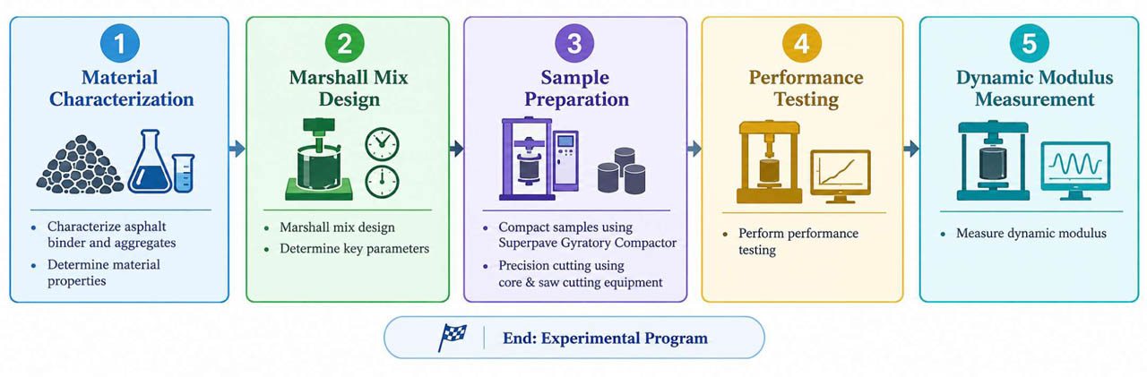
Figure 1:
Experimental program to acquire data for predicting dynamic modulus
3.1. Materials
The locally sourced limestone aggregates obtained from Pakistan were used as the aggregate material in the bituminous mixtures. To characterize their fundamental properties, a series of laboratory tests were performed, including soundness (durability), sand equivalent value, elongation index, flakiness index, and Los Angeles abrasion. All laboratory tests were conducted in accordance with the applicable national standards. The results of these tests are presented in Table 1. Based on the measured aggregate properties, sixteen different gradation blends (GB) were developed and designated as GB-1 to GB-16, as shown in Table 2.
Table 1:
Key properties of aggregates
| Aggregate Property | Reference Standard | Average Value [%] | Value Range [%] |
|---|---|---|---|
| Soundness | AASHTO T104 | 3 | ≤12 |
| Sand Equivalent Value | AASHTO T 176 | 72 | ≥ 45 |
| Elongation Ratio | ASTM D 4791 | 7 | ≤ 10 |
| Flakiness Ratio | ASTM D 4791 | 5 | ≤ 10 |
| Los Angeles Abrasion | AASHTO T96 | 26 | ≤ 30 |
Table 2:
Gradation blend details
| Gradation Blend | Sieve Size [mm]/Percent Passing [%] | ||||||||
|---|---|---|---|---|---|---|---|---|---|
| 37.5 | 25.0 | 19.0 | 12.5 | 9.5 | 4.75 | 2.36 | 0.30 | 0.075 | |
| GB-1 | - | - | - | 82.5 | 68.7 | 49.3 | 30.8 | 10.5 | 5.2 |
| GB-2 | - | - | 99.9 | 79.5 | 69.4 | 48.7 | 35.3 | 11.8 | 5.2 |
| GB-3 | - | - | 99.7 | 84.5 | 63.4 | 46.0 | 30.5 | 10.3 | 5.0 |
| GB-4 | - | - | - | 80.0 | 67.0 | 48.0 | 33.0 | 11.0 | 4.7 |
| GB-5 | - | 82.6 | 69.7 | 59.2 | 52.2 | 41.6 | 24.5 | 9.4 | 5.0 |
| GB-6 | - | 85.4 | 71.0 | 59.9 | 53.4 | 35.5 | 26.4 | 10.8 | 4.7 |
| GB-7 | 98.8 | 82.7 | 67.4 | 56.2 | 43.5 | 35.0 | 25.1 | 7.6 | 4.2 |
| GB-8 | - | - | 95.0 | 76.0 | 63.0 | 42.5 | 29.0 | 8.5 | 5.0 |
| GB-9 | - | - | - | 82.0 | 70.0 | 50.0 | 30.0 | 10.0 | 5.0 |
| GB-10 | - | - | - | 94.0 | 87.0 | 65.0 | 37.0 | 9.0 | 5.0 |
| GB-11 | - | - | - | 95.0 | 82.0 | 59.0 | 43.0 | 13.0 | 6.0 |
| GB-12 | 95.0 | 77.0 | 65.5 | 52.5 | 44.0 | 31.5 | 22.5 | 7.0 | 4.5 |
| G-13 | - | 82.5 | 72.5 | 62.5 | 52.5 | 37.5 | 25.0 | 10.0 | 4.5 |
| GB-14 | - | 95.0 | 85.0 | 60.0 | 47.0 | 30.0 | 20.0 | 8.0 | 4.0 |
| GB-15 | - | 95.0 | 83.0 | 70.0 | 63.0 | 52.0 | 39.0 | 14.0 | 5.5 |
| GB-16 | - | - | 95.0 | 83.0 | 65.0 | 46.0 | 30.0 | 9.0 | 5.0 |
There are two main suppliers of bitumen in Pakistan, namely Attock Refinery Limited (ARL) and National Refinery Limited (NRL). Four bitumen grades were obtained from these two suppliers and used to prepare the asphalt mixtures. Standard laboratory tests, including penetration, softening point, flash and fire points, and viscosity, were conducted to determine the physical and rheological characteristics of the binders. The results are presented in Table 3. ARL 40/50 was identified as the hardest binder grade among the tested samples based on its lowest penetration value, followed by NRL 60/70, ARL 60/70, and ARL 80/100. The viscosity results further indicated that ARL 40/50 had the highest resistance to flow, whereas ARL 80/100 exhibited the lowest viscosity and, consequently, the greatest ease of handling at the specified testing temperatures. The observed viscosity trends are consistent with the expected relationship between asphalt penetration grade, viscosity, flow behavior, and workability.
Table 3:
Key properties of bitumen
| Bitumen Property | Reference Standard | ARL 40/50 | ARL 80/100 | ARL 60/70 | NRL 60/70 |
|---|---|---|---|---|---|
| Penetration Value [0.1 mm] | AASHTO T49 | 43 | 84 | 66 | 64 |
| Softening Point [°C] | AASHTO T53 | 52 | 46 | 48.8 | 49.2 |
| Flash and Fire Points [°C] | AASHTO T48 | 335 & 359 | 233 & 275 | 304 & 334 | 310 & 343 |
| Viscosity at 135°C [ Pa·s] | AASHTO T316 | 0.486 | 0.226 | 0.241 | 0.292 |
As mentioned earlier, the study included 16 aggregate gradations and four binder types, with the latter differing in either penetration grade or source. The experimental matrix was compiled by combining data from two independent experimental projects. The first project focused on evaluating the effects of different asphalt grades using a limited number of aggregate gradations, whereas the second investigated the effects of different aggregate gradations using 60/70 penetration-grade asphalt, which is commonly used for pavement applications in Pakistan. In the second project, the binder was obtained from a different source because of material availability; however, the relevant binder properties were comparable, as shown in Table 3. Consequently, the available dataset constitutes a partially crossed and unbalanced experimental matrix, in which not all combinations of aggregate gradations and binder types were available. Table 4 summarizes the gradation subsets tested with each binder type. Across all available combinations, a total of 576 asphalt mixtures were evaluated for DM. Each mixture was tested using 24 specimens across different temperature and loading-frequency conditions. Four temperature levels and six loading frequencies were considered, resulting in a full factorial temperature–frequency design of 4T×6f for each mixture.
Table 4:
Summary of mix design parameters using the Marshall method
| Bitumen Source/Type | Gradation Blend | Air Voids [%] | Optimum Binder Content [%] | Voids in Mineral Aggregate [%] | Voids Filled with Asphalt [%] | Stability [Kg] | Flow [mm] |
|---|---|---|---|---|---|---|---|
| ARL 40/50 | G-8 | 4.0 | 3.9 | 13.09 | 69.44 | 1198 | 2.29 |
| G-10 | 4.0 | 5.5 | 15.22 | 73.71 | 1447 | 2.63 | |
| G-14 | 4.0 | 3.4 | 13.16 | 69.62 | 2243 | 3.40 | |
| G-15 | 4.0 | 4.4 | 13.55 | 70.48 | 3114 | 9.00 | |
| ARL 80/100 | G-8 | 4.0 | 3.7 | 11.32 | 64.66 | 790 | 2.68 |
| G-10 | 4.0 | 4.6 | 15.04 | 73.40 | 934 | 2.58 | |
| G-14 | 4.0 | 3.3 | 11.45 | 65.07 | 2526 | 8.81 | |
| G-15 | 4.0 | 4.3 | 12.30 | 67.50 | 610 | 7.52 | |
| ARL 60/70 | G-3 | 4.0 | 4.2 | 14.20 | 66.50 | 1343 | 3.10 |
| G-4 | 4.0 | 4.2 | 13.40 | 59.50 | 1298 | 2.99 | |
| G-7 | 4.0 | 3.5 | 12.80 | 58.00 | 2632 | 5.02 | |
| G-8 | 4.0 | 4.0 | 12.15 | 66.08 | 1362 | 3.00 | |
| G-9 | 4.0 | 4.1 | 12.95 | 65.16 | 1291 | 3.16 | |
| G-10 | 4.0 | 5.0 | 14.70 | 69.18 | 1424 | 3.38 | |
| G-11 | 4.0 | 4.8 | 14.52 | 67.73 | 1544 | 3.28 | |
| G-12 | 4.0 | 3.3 | 11.38 | 62.19 | 2650 | 4.81 | |
| G-13 | 4.0 | 3.7 | 11.87 | 63.33 | 2905 | 4.66 | |
| G-14 | 4.0 | 3.6 | 12.17 | 61.93 | 2295 | 5.38 | |
| G-15 | 4.0 | 3.9 | 12.40 | 61.33 | 3496 | 4.53 | |
| G-16 | 4.0 | 4.36 | 14.43 | 74.53 | 3235 | 9.12 | |
| NRL 60/70 | G-1 | 4.0 | 4 | 14.8 | 66.9 | 1290 | 2.88 |
| G-2 | 4.0 | 4.4 | 15.3 | 63.5 | 1330 | 3.052 | |
| G-5 | 4.0 | 3.3 | 13.7 | 58.1 | 2890 | 4.302 | |
| G-6 | 4.0 | 3.4 | 13.2 | 59.2 | 2620 | 4.981 |
3.2. Mix Design
The Marshall method, conducted in accordance with ASTM D6927, was employed to design the HMA mixtures and determine the corresponding mix-design parameters for the selected aggregate gradations and bitumen types. The resulting Marshall mix-design parameters, including OBC, Va, VMA, VFA, stability, and flow, are presented in Table 4. For each gradation–bitumen combination, HMA specimens were prepared using several bitumen content levels, as illustrated in Figure 2, to establish the relationships required for determining the OBC. Specimen compaction was performed by applying 75 blows to each face of the specimen to ensure consistent and uniform compaction, while maintaining the compaction temperature at 145 ± 5 °C. Following compaction and subsequent Marshall testing, the OBC for each gradation–bitumen combination was determined based on the specified Marshall mix-design criteria.
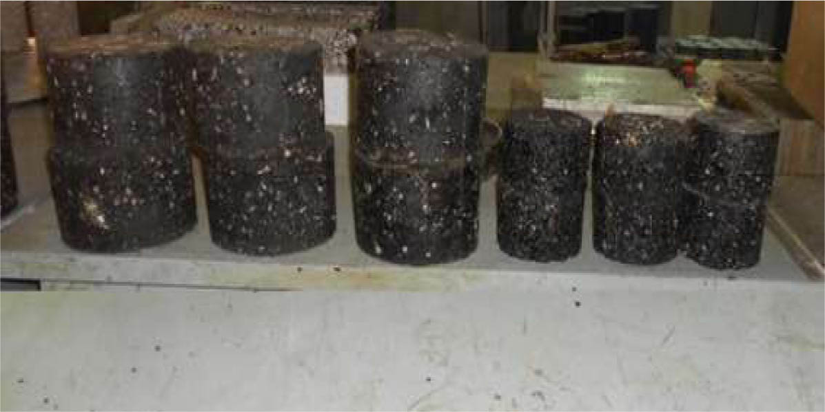
Figure 2:
Representative HMA specimens at different bitumen contents
The OBC values reported in Table 4 were then used as the binder contents for preparing the corresponding HMA specimens for DM testing. The resulting HMA specimens were compacted using a SGC to achieve the specified compaction density. After cooling to room temperature, the specimens were cored and trimmed to a diameter of 100 mm and a height of 150 mm to satisfy the dimensional requirements of the DM test, as shown in Figure 3 (Han et al., 2021a).
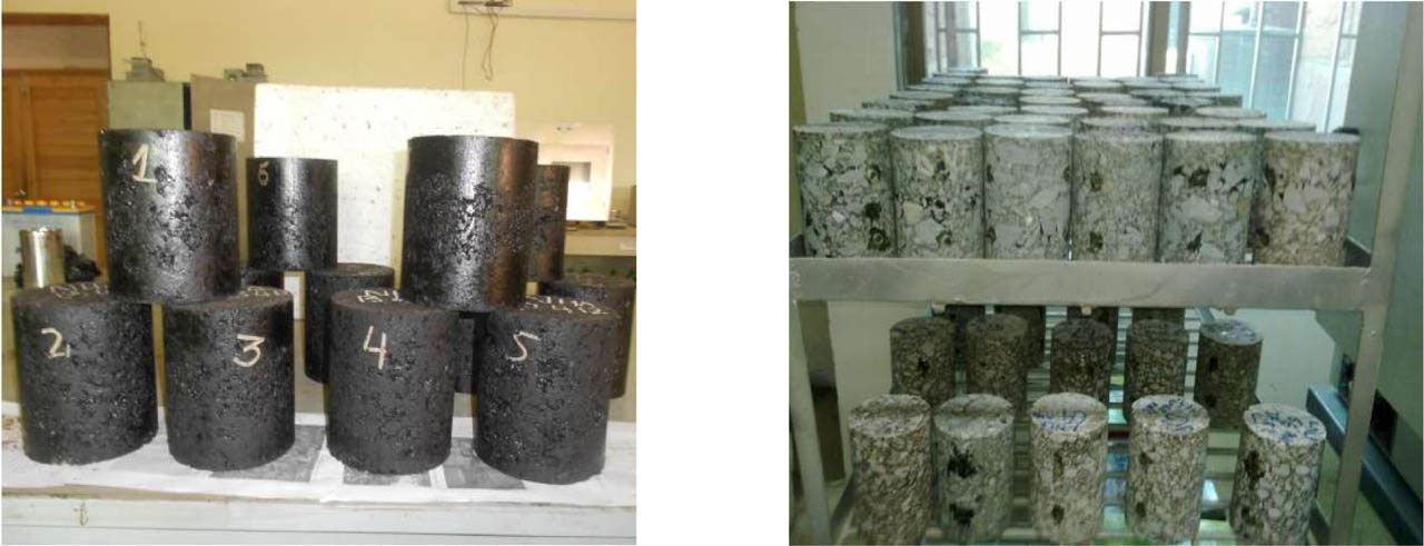
Figure 3:
Core and uncore specimens for dynamic modulus testing
3.3. Laboratory Testing
The DM characterizes the relationship between stress and strain in a linear viscoelastic material subjected to sinusoidal loading. The phase angle represents the time lag between the applied stress and the resulting recoverable axial strain, with values near zero degrees indicating a predominantly elastic response and values approaching ninety degrees indicating a predominantly viscous response (Bonaquist, 2008). To characterize the viscoelastic response of the asphalt mixtures, DM and phase angle were measured using the Simple Performance Tester (SPT), which applies cyclic axial loading at specified frequencies. The mixtures were evaluated at temperatures of 4.4, 21.1, 37.8, and 54.4 °C and loading frequencies of 25, 10, 5, 1, 0.5, and 0.1 Hz. Before each test, the specimens were conditioned until thermal equilibrium was reached at the specified temperature, after which DM and phase angle were recorded for each temperature-frequency combination.
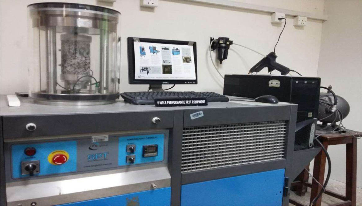
Figure 4:
Conducting SPT on a cored sample
4. Modelling Method
4.1. Overview of Modeling Framework
A significant dataset was generated from the experimental program described in the previous section, comprising DM measurements obtained under different temperature and loading frequency conditions, together with corresponding mix-design parameters, including aggregate gradation, binder type, and volumetric properties. Given the nonlinear and viscoelastic behavior of asphalt mixtures, these variables may interact in complex ways, requiring advanced modeling approaches to accurately predict DM (Junaid et al., 2025). Accordingly, eight models were developed, including Linear Regression (LR), Interaction Linear Regression (ILR), Fine Tree (FT), Medium Tree (MT), Quadratic Support Vector Machine (QSVM), Cubic Support Vector Machine (CSVM), Ensemble Boosted Trees (EBT), and Ensemble Bagged Trees (EBagT). These models represent a range of learning approaches, from conventional parametric regression to nonlinear and ensemble-based methods. All models were developed using the MATLAB Regression Learner application, which was used for predictor standardization, model training, 10-fold cross-validation, model comparison, and final performance evaluation.
4.2. Model Configuration and Hyperparameters
Machine-learning models were developed using the MATLAB Regression Learner application (MATLAB R2024b). Eight regression models were considered, including LR, ILR, FT, MT, QSVM, CSVM, EBT, and EBagT. The configurations of these models used in the MATLAB Regression Learner environment are summarized in Table 5.
Table 5:
Model configurations and hyperparameters used in the MATLAB Regression Learner application
| Model | MATLAB function | Model specification | Main settings |
|---|---|---|---|
| LR | fitlm | Linear regression | RobustOpts = off |
| ILR | fitlm | Interaction regression | RobustOpts = off |
| FT | fitrtree | Fine regression tree | MinLeafSize = 4; Surrogate = off |
| MT | fitrtree | Medium regression tree | MinLeafSize = 12; Surrogate = off |
| QSVM | fitrsvm | Quadratic polynomial SVM | PolynomialOrder = 2; KernelScale = auto; BoxConstraint = IQR/1.349; Epsilon = IQR/13.49; Standardize = true |
| CSVM | fitrsvm | Cubic polynomial SVM | PolynomialOrder = 3; KernelScale = auto; BoxConstraint = IQR/1.349; Epsilon = IQR/13.49; Standardize = true |
| EBT | fitrensemble | LSBoost | 30 learning cycles; LearnRate = 0.1; tree MinLeafSize = 8; variables sampled = all |
| EBagT | fitrensemble | Bagging | 30 learning cycles; tree MinLeafSize = 8; variables sampled = all |
For the Support Vector Machine (SVM) models, the QSVM and CSVM employed polynomial kernels of order 2 and 3, respectively. The kernel scale was determined automatically by MATLAB, while the Box Constraint and epsilon-insensitive loss parameters were calculated from the interquartile range (IQR) of the response variable according to (IQR(DM)/1.349) and (IQR(DM)/13.49), respectively. Predictor standardization was enabled for both SVM models. For the tree-based models, the FT and MT used minimum leaf sizes of 4 and 12, respectively, with surrogate splits disabled. The EBT model employed the LSBoost method with 30 learning cycles and a learning rate of 0.1, using regression trees with a minimum leaf size of 8. The EBagT model employed the Bag method with 30 learning cycles and the same base-tree configuration. For both ensemble models, all predictor variables were available for sampling at the tree splits. All models were evaluated using 10-fold cross-validation within the training dataset. No, separate grid-search or Bayesian hyperparameter optimization procedure was used; instead, the model configurations were specified and implemented within the MATLAB Regression Learner environment.
4.3. Data Processing, Distribution, and Statistical Characteristics
Prior to developing predictive models, the dataset was processed to ensure consistent formatting and suitability for machine-learning applications. The input attributes included aggregate gradation characteristics, binder properties, volumetric attributes, and test conditions, while the target attribute was the DM measured during laboratory testing. Although temperature has a strong influence on the DM of HMA, it was not included as a direct predictor in the machine-learning models. Instead, binder viscosity was used to represent the temperature-related effect because it is strongly dependent on temperature and directly reflects the temperature-dependent rheological response of the binder. Temperature was therefore intentionally excluded as a separate predictor to avoid redundancy with the viscosity-related input and maintain a consistent representation of the temperature-dependent binder response. The numerical predictor variables were standardized using the “Standardize Data” option in the MATLAB Regression Learner application to place them on a common scale and improve numerical stability when variables have different units and magnitudes. The complete dataset was then randomly partitioned using the MATLAB Regression Learner application, with 70% of the observations assigned to the training dataset and the remaining 30% retained as an independent testing dataset. The training subset was used for model development, while the testing subset was kept separate from the training and validation procedures and used only for final independent performance evaluation. Within the training subset, 10-fold cross-validation was employed in MATLAB Regression Learner, whereby the training data were divided into ten folds, with each fold used sequentially for validation while the remaining nine folds were used for model training. This procedure was applied consistently to all machine learning models to assess their generalization performance and reduce the possibility of overfitting.
The dataset's statistical distribution is shown in Figure 5, which presents the histograms of the key input variables as well as the target output. The viscosity values show distinct variations among the four binder types used in the study. Considerable variability was also observed in the aggregate gradation parameters, with P200 ranging from approximately 4.0% to 6.0%, P4 from 45% to 70%, and P3/8 varying by as much as 35%. The phase angle ranged from approximately 5° to 45°, with a large proportion of samples falling between 20° and 35°, indicating variation in the viscoelastic behavior of the binder under different conditions. The frequency values were discrete, with most samples tested at the lower end of the frequency spectrum (0–5 Hz) and a smaller number tested at higher frequencies near 10 and 25 Hz. Vbeff ranged from approximately 3.2% to 5.5%, with a concentration of observations between 3.8% and 4.4%, while Va values were closely grouped around 4.0%, suggesting that the mix designs were well controlled. Overall, the DM values were widely dispersed and left-skewed, with a high concentration of values at or below 2,000,000 psi and maximum values reaching approximately 5,000,000 psi. These distributions provide a balance between variability and control, supporting the development of a robust predictive model capable of predicting DM across a wide range of conditions.
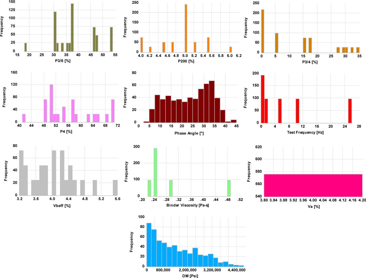
Figure 5:
Histogram matrix showing the frequency distributions of key material and rheological parameters
4.4. Spearman Correlation Analysis
To determine the relationships among the input parameters and understand how they affect DM, a Spearman Rank Correlation Analysis was performed, as illustrated in Figure 6. Spearman's Coefficient (ρ) is used to analyze monotonic relationships without assuming linearity and to identify potential nonlinear associations in the complex behavior of asphalt mixtures. The results indicate very strong relationships among the aggregate gradation parameters. In particular, a very strong inverse relationship was observed between P200 and P4 (ρ = − .89), suggesting that an increase in the fine fraction is associated with a decrease in the intermediate aggregate fraction. A positive association was also observed between P200 and Vbeff (ρ = .64), indicating that a higher fine fraction is associated with a higher effective binder volume. In addition, positive associations were found between P4 and P3/8 (ρ = .80), and between P3/8 and P3/4 (ρ = .83), indicating that different aggregate fractions tend to vary in a consistent manner, consistent with local and international design practices.
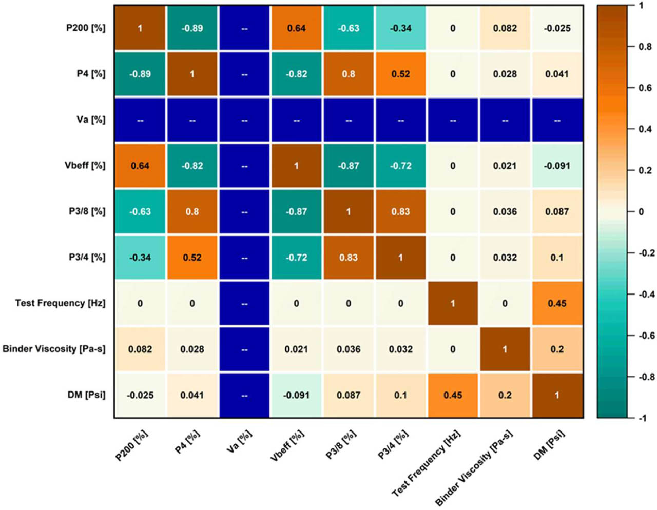
Figure 6:
Spearman Correlation matrix heatmap showing relationships among mixture components
The relationships between the individual input factors and DM were generally weak to moderate. Testing Frequency showed the strongest relationship with the DM (ρ=0.45), followed closely by Binder Viscosity (ρ=0.20). The remaining factors, including P3/4 (ρ=0.10) and P200 (ρ=−0.025), showed very weak to negligible correlations with the DM. Va exhibited virtually no correlation, which was expected since the Marshall mix design process focuses on maintaining approximately 4% Va. suggest that the input variables may have complex interactions; although most variables exhibit relatively weak individual associations with DM, they may not operate independently and could jointly influence DM through their interactions with one another.
Traditional empirical methods, such as the Witczak model, are generally limited in their ability to capture such complex, higher-order interactions because they rely on predefined functional forms. The observed relationships therefore provide further motivation for employing machine learning algorithms capable of capturing complex nonlinear associations. Kernel-based methods such as SVM can capture complex nonlinear associations without requiring them to be explicitly formulated. The following section presents the modeling approaches adopted in this study.
4.5. Linear Regression Models
LR was used as a baseline model to provide a benchmark. The LR model assumes that the dependent variable is related to one or more independent variables through a linear function given in Equation (3):
Where:β0- intercept,
βi- array of model coefficients,
Xi- array of input variables.
LR models are simple and easy to interpret; however, they do not perform well when modeling complex, nonlinear relationships. To address this limitation, ILR was created and extended with all possible pairwise interactions as shown in Equation (4):
Where:β0, βi - as defined earlier,
Xi- main effect term,
Xi,Xj- interaction effect term.
These additional features enable ILR models to capture the coupled effects of the independent variables on the output, thus allowing them to make more accurate predictions than LR models, while maintaining the same level of interpretability.
4.6. Decision Tree Models
Decision trees divide the input data into discrete areas or "regions" and use a single prediction for all points within each region. Decision tree models can be represented by Equation (5):
Where:Rm - terminal regions (or leaf nodes) (where (m = 1, 2, …., M),
cm - constant predicted value.
An FT model uses an excessive number of splits to capture highly specific patterns in the data, which may lead to overfitting, whereas an MT model provides a balance between model complexity and generalizability. Decision trees can capture nonlinear relationships; however, they cannot capture smooth variations in the response because of their discontinuous nature.
4.7. Support Vector Machine Models
A general regression function utilizing SVM for modeling nonlinear relationships with a kernel-based approach was employed using Equation (6).
Where:X - the new input data,
Xi - historical training data points (i = 1, 2, 3, ….., N),
- Lagrange multiplier,
K(Xi, X)- the kernel function,
b - bias.
The Quadratic and Cubic versions of the SVM used in this study are based on quadratic and cubic polynomials, respectively. The Quadratic SVM uses the kernel shown in Equation (7), while the Cubic SVM uses the kernel function shown in Equation (8):
These kernels allow the input data to be mapped into higher-dimensional spaces, enabling the models to identify and capture complex nonlinear interactions among the input variables, as suggested by the correlation analysis.
4.8. Ensemble Learning Models
Ensemble methods were used to combine multiple learners to improve prediction accuracy by employing EBagT and EBT models. The EBagT model is trained using multiple decision trees on bootstrap resamples, with the final prediction obtained by averaging their predictions. On the other hand, EBT trains a series of sequential models to minimize residual errors (Equation (9)):
Where:X - the input feature,
hm (X) - the base learner/individual tree,
γm - tree weight/shrinkage factor,
M – total trees build in the ensemble,
The combination of trees in these methods improves model robustness and reduces variance compared with single tree models.
4.9. Model Evaluation
The predictive performance of all models was evaluated using statistical metrics. The coefficients of determination (R2) were used to assess how well each model fit the data. In addition, the root mean squared errors (RMSE), the mean squared errors (MSE), and the mean absolute errors (MAE) were calculated. Overall, these metrics enabled comparison of the machine learning models in terms of predictive accuracy, prediction error, and generalization ability. In addition to evaluating predictive performance, the models were used to examine the effects and relationships of the input variables on DM using SHapley Additive exPlanations (SHAP), a widely used method for explaining machine learning models based on cooperative game theory, which quantifies the contribution of each variable to individual predictions across the dataset (Bernal et al., 2025).
5. Results and Discussion
Building upon the correlation analysis presented in Section 4.3, which revealed weak individual relationships and strong interdependencies among variables, this section evaluates the ability of different models to capture the complex nonlinear behavior governing DM.
5.1. Model Performance
The predictive accuracy of the models developed was assessed for both the test data and validation data, as shown in Table 6. A significant difference in model capabilities was observed, primarily due to each model's ability to represent the nonlinear interactions inherent in asphalt mixture behavior. The LR Model provided an R2 of 0.90 and an RMSE of 3.64 x 10⁵ psi, indicating that its linear representation provides a poor approximation of the complex viscoelastic behavior. The ILR model demonstrated a significant improvement, providing a better R2 (0.94), and a reduced RMSE (2.78 x 10⁵ psi), demonstrating the importance of including interaction terms among factors such as temperature, loading frequency, and volumetrics.
Table 6:
Metric analysis results for all models
| Model | RMSE [psi] (Validation) | MSE [psi2] (Validation) | R2 [-] (Validation) | MAE [psi] (Validation) | MAE [psi] (Test) | MSE [psi2] (Test) | RMSE [psi] (Test) | R2 [-] (Test) |
|---|---|---|---|---|---|---|---|---|
| LR | 3.87 × 10⁵ | 1.50 × 10¹¹ | 0.86 | 3.00 × 10⁵ | 2.93 × 10⁵ | 1.32 × 10¹¹ | 3.64 × 10⁵ | 0.90 |
| ILR | 3.22 × 10⁵ | 1.03 × 10¹¹ | 0.90 | 2.32 × 10⁵ | 2.05 × 10⁵ | 7.78 × 10¹⁰ | 2.78 × 10⁵ | 0.94 |
| FT | 3.97 × 10⁵ | 1.58 × 10¹¹ | 0.85 | 3.11 × 10⁵ | 2.86 × 10⁵ | 1.49 × 10¹¹ | 3.86 × 10⁵ | 0.89 |
| MT | 4.37 × 10⁵ | 1.91 × 10¹¹ | 0.82 | 3.38 × 10⁵ | 2.86 105 | 1.46 × 10¹¹ | 3.82 × 10⁵ | 0.89 |
| QSVM | 2.78 × 10⁵ | 7.73 × 10¹⁰ | 0.93 | 1.96 × 10⁵ | 1.80 × 10⁵ | 6.18 × 10¹⁰ | 2.48 × 10⁵ | 0.95 |
| CSVM | 2.32 × 10⁵ | 5.39 × 10¹⁰ | 0.95 | 1.67 × 10⁵ | 1.51 × 10⁵ | 4.90 × 10¹⁰ | 2.21 × 10⁵ | 0.96 |
| EBT | 3.11 × 10⁵ | 9.67 × 10¹⁰ | 0.91 | 2.40 × 10⁵ | 2.08 × 10⁵ | 7.99 × 10¹⁰ | 2.82 × 10⁵ | 0.94 |
| EBagT | 3.42 × 10⁵ | 1.17 × 10¹¹ | 0.89 | 2.55 × 10⁵ | 2.21 × 10⁵ | 8.73 × 10¹⁰ | 2.95 × 10⁵ | 0.93 |
The decision tree models showed a relatively lower predictive capability compared to other models. The FT model resulted in an R2 value of 0.89 and an RMSE of 3.86 x 10⁵ psi. The MT model also had an R2 value of 0.89 and an RMSE of 3.82 x 10⁵ psi. This shows that individual tree-based approaches are generally less capable of describing continuous nonlinear patterns because of the discrete and piecewise nature of each tree. Combining multiple trees into an ensemble model improves predictive performance through reduced variability and increased stability. The EBT model had an R2 value of 0.94 and an RMSE of 2.82 x 10⁵ psi. The EBagT model achieved an R2 value of 0.93 with an RMSE of 2.95 x 10⁵ psi.
The highest predictive performance was achieved by the SVM. The Quadratic SVM produced an R2 value of 0.95 and an RMSE of 2.48 x 10⁵ psi. However, the Cubic SVM had the highest R2 (0.96) and the lowest RMSE (2.21 x 10⁵ psi), as well as the lowest MAE (1.51 x 10⁵ psi). Therefore, the Cubic SVM model provided more than 30% improvement over the single tree and regression models, demonstrating that high order nonlinear models can be very effective with the randomly applied dataset split scheme of cross-validation. The accuracies accuracies achieved in this study represent a substantial improvement over those obtained using the Witczak models on the same dataset by Junaid et al. (2025). The current study is an extension of the aforementioned study; hence, it adopts a similar methodology for model calibration. Compared with the Witczak models, the AI models in the current study achieved approximately 60% higher accuracy in terms of R2, indicating that they may be more suitable for explainable analysis. The comparison with other accuracy parameters was not done because the Witczak models are traditionally designed to predict logE*, whereas the AI models in this study directly predict DM. Hence, a direct comparison of these accuracy parameters was not performed to avoid potential distortion in the reported results.
5.2. Predicted vs Actual Analysis
Figure 7 displays the overall accuracy, reliability, and generalizability of the models for DM by comparing predicted values with measured values. Data point alignment on or near the equality line is an important factor in determining whether the predictive models are accurate, while the spread and distribution of the points help identify potential bias and variability in the models. A group of closely clustered points around the 1:1 equality line typically demonstrates good accuracy and little dispersion, and vice versa. The proximity of the points to the equality line also indicates the model's ability to represent relationships among variables.
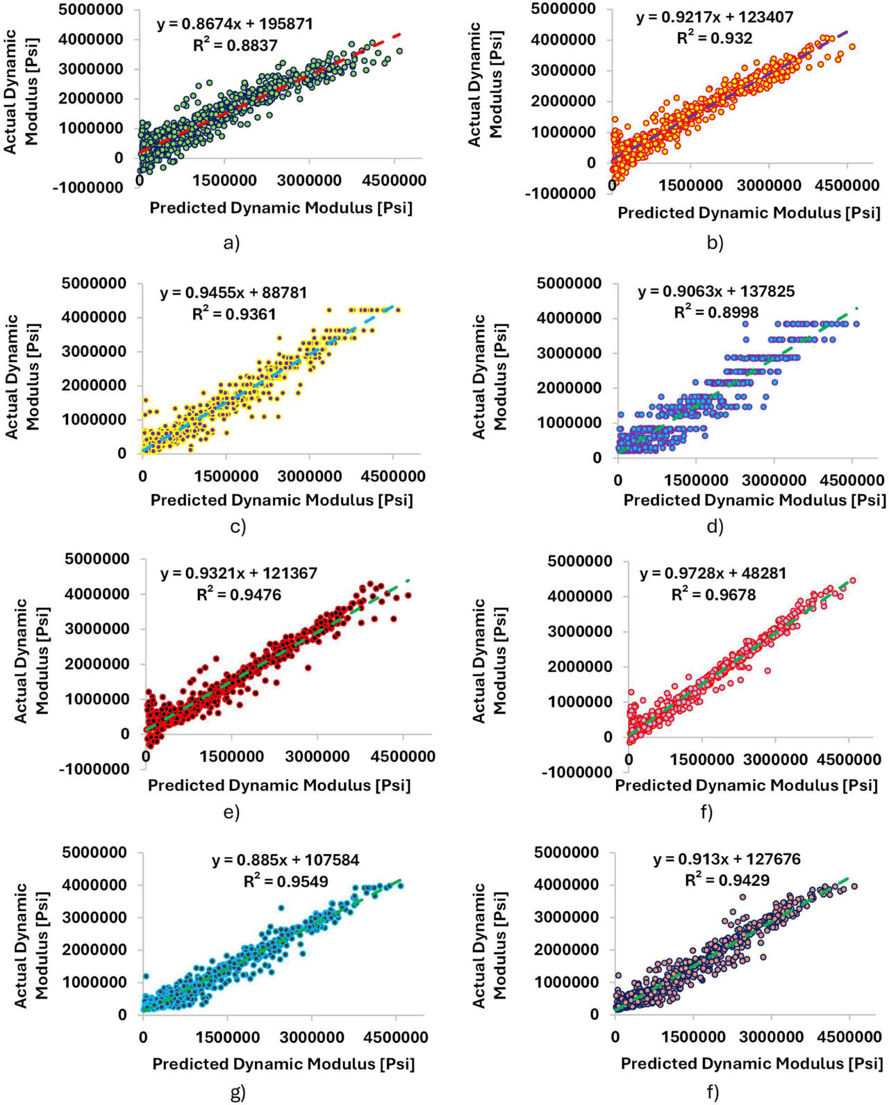
Figure 7:
Actual vs predicted dynamic modulus (Psi) a) LT b) ILT c) FT d) MT e) QSVM f) CSVM g) EBT h) EBagT
The LR model exhibits a significant amount of scatter about the line of equality as the DM increases, which is also reflected in it having an approximate R2 value of 0.90. This behaviour is indicative of systematic underfitting, suggesting that this model does not include enough nonlinear terms to describe how materials respond under various stimuli. The ILR, compared with LR, appears to be much better aligned and exhibits less scatter in the data, as indicated by its approximate R2 value of 0.93. Therefore, the inclusion of interaction effects improves model fit; however, other types of nonlinear interactions may also be present and are not fully captured by the current model.
The piece-wise predictive nature of the decision tree models is reflected in different clusterings of the predicted values. The FT model (R2 = ~ 0.93) displays a moderate level of alignment with the data but exhibits a noticeable “step-like” distribution in its predictions. This indicates that the FT model produces discrete predictions. The MT model (R2 = ~ 0.90) shows greater variability and lower homogeneity compared with the FT model, especially for higher modulus values. In this context, both the FT and MT models indicate the limitations of using a single tree for modelling the smooth viscoelastic behaviour and capturing continuous variations.
The ensemble models show better performance than the individual decision tree models. Both the EBT (R2 = ~ 0.95) and EBagT (R2 = ~ 0.94) exhibit tighter clustering and lower variability than either of the previous two models. The combination of multiple trees also improves prediction stability and reduces variability across runs. However, small discrepancies remain in both ensemble models, although these seem to be limited primarily to the higher ranges of the dataset.
The SVM models showed a stronger correlation with the experimental results than the other models examined. The QSVM model achieved an R2 value of approximately 0.95 and showed good correspondence throughout the entire dataset. In addition, the CSVM model achieved an R2 value of approximately 0.96 and demonstrated an excellent fit with minimal scatter around the best-fit curve. Furthermore, CSVM model maintained this high degree of accuracy over the entire range of modulus values, including extreme values, where some models deviated significantly from the expected relationship. It is also important to note that a uniform distribution of points on either side of the line of equality indicates a low degree of bias and, therefore, suggests good generalizability for these types of models. Therefore, these findings suggest that SVM models can be effective in capturing the complex nonlinear relationships associated with DM under varying temperatures and loading conditions. However, this argument needs further validation with varying dataset split mechanisms for cross-validation.
Using phase angle to predict dynamic modulus has potential for data-leakage and circular-prediction issues. Hence, an additional sensitivity analysis was conducted by excluding phase angle from the input variables to evaluate the predictive capability of the models using the remaining mixture and testing-condition parameters. The models were developed using MATLAB Regression Learner with the same 70/30 training–testing framework and 10-fold cross-validation procedure used in the original analysis. All other aspects of the model-development procedure were retained, with phase angle being the only excluded predictor.
The results demonstrate a substantial reduction in predictive performance when phase angle is excluded as shown in Table 7 and comparison of modelled developed with Phase angle and no phase angle is shown in Table B. For the Cubic SVM model, for example, the test (R2) decreased from 0.96 with phase angle to −0.18 without phase angle, while the corresponding test RMSE increased from approximately (2.21 × 10⁵) psi to (1.16 × 10⁶) psi. Similar reductions in predictive performance were observed for the other models. In the phase-angle-excluded analysis, the test (R2) values ranged from −0.2180 to 0.0704.
Table 7:
Sensitivity Analysis for phase angle
| Model | Phase Angle [-] | No-Phase Angle [-] | Phase Angle RMSE [psi] | No-Phase Angle RMSE [psi] |
|---|---|---|---|---|
| LR | 0.90 | 0.0704 | 3.64 × 10⁵ | 1.03 x 10⁶ |
| ILR | 0.94 | 0.0636 | 2.78 × 10⁵ | 1.03 x 10⁶ |
| FT | 0.89 | −0.2180 | 3.86 × 10⁵ | 1.17 x 10⁶ |
| MT | 0.89 | −0.0855 | 3.82 × 10⁵ | 1.11 x 10⁶ |
| QSVM | 0.95 | −0.0219 | 2.48 × 10⁵ | 1.07 x 10⁶ |
| CSVM | 0.96 | −0.1854 | 2.21 × 10⁵ | 1.16 x 10⁶ |
| EBT | 0.94 | 0.0150 | 2.82 × 10⁵ | 1.05 x 10⁶ |
| EBagT | 0.93 | 0.0262 | 2.95 × 10⁵ | 1.05 x 10⁶ |
These results indicate that phase angle provides substantial predictive information for dynamic modulus within the present dataset and experimental conditions. The findings are also consistent with the SHAP analysis, which identified phase angle as the most influential predictor in the original Cubic SVM model.
5.3. Model Interpretability Analysis with Feature Importance
The feature importance analysis based on SHAP values for the cubic SVM is provided in Figure 8. It shows the extent to which each input variable contributed to predicting DM. The results clearly reveal a hierarchy of parameter influence, with phase angle being the most dominant variable, with a mean SHAP value of approximately 1.05 x 10⁶. This substantially larger contribution than those of the other variables highlights the importance of viscoelastic behavior in determining mixture stiffness.
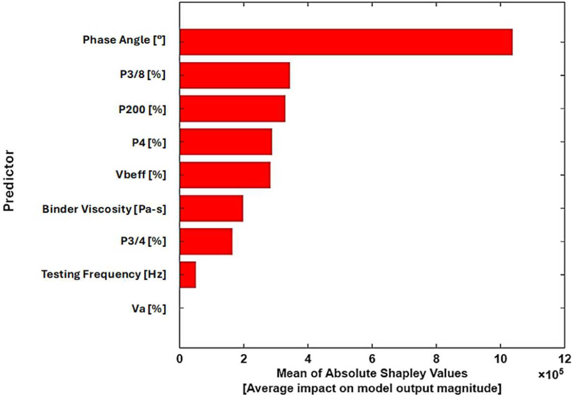
Figure 8:
Shapley feature importance analysis for Model [Cubic SVM]
The two parameters of the aggregate gradation that have a very significant effect on the model output are P3/8 and P200, with SHAP values of around 3.4 x 10⁵ and 3.2 x 10⁵, respectively. The next most influential parameters in the prediction model are P4 and Vbeff, with SHAP values of approximately 2.8 x 10⁵ and 2.7 x 10⁵, respectively. Binder viscosity is also highly influential, with a SHAP value of approximately 2.1 x 10⁵, while P3/4 has a moderate influence, with a SHAP value of approximately 1.7 x 10⁵, on the model predictions. Testing frequency has relatively little influence, with a SHAP value of approximately 0.4 x 10⁵, while Va has no significant influence on the model predictions.
The SHAP summary plot in Figure 9 also shows the variation in feature effects across individual samples in the dataset. As shown by the wide range of SHAP values (approximately −1.5 x 10⁶ to +3.5 x 10⁶), there is a high level of variability among the tested samples in terms of their sensitivity to changes in phase angle. Lower phase angles make positive contributions to DM predictions, whereas higher phase angles result in significant reductions in predicted DM. Similar patterns were observed for aggregate parameters (e.g., P3/8 and P200), with consistent contributions to the model predictions across their respective ranges. Test frequency and Va showed relatively low variability and remained centered around zero SHAP value, indicating that they had little or no influence on the predictions.
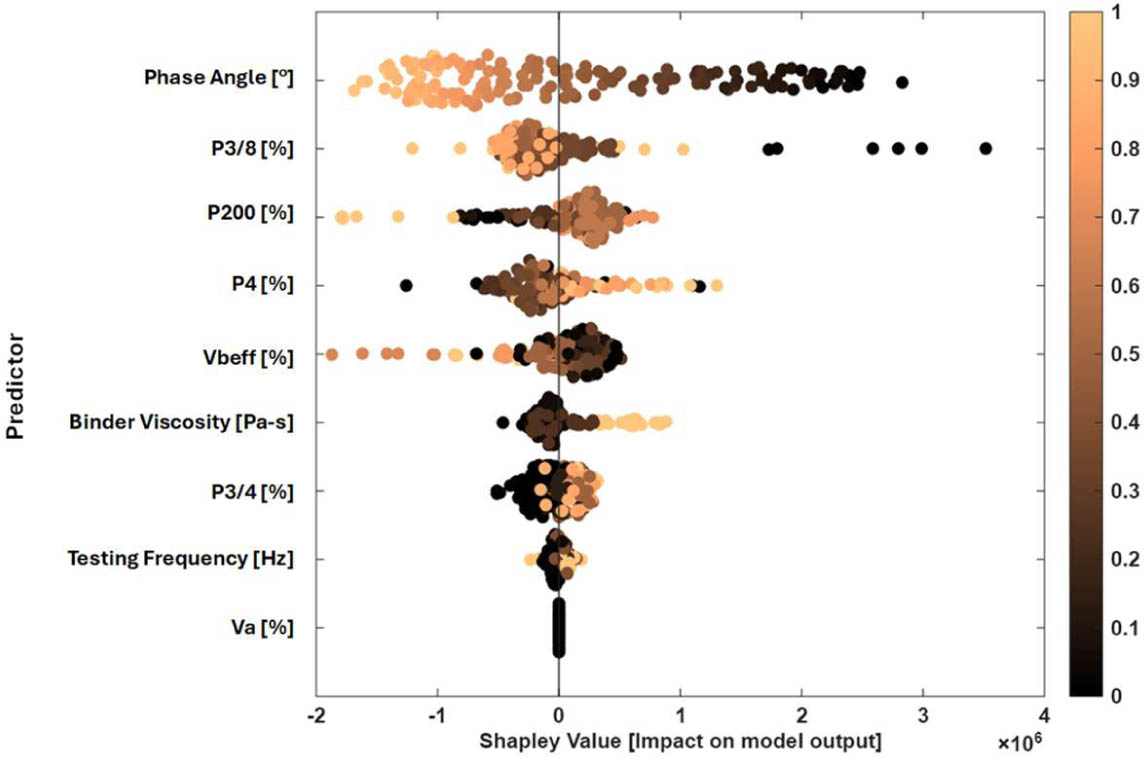
Figure 9:
SHAP summary plot for the Cubic SVM model
The SHAP dependency plot, as depicted in Figure 10, reveals further information on how specific variables' impacts on prediction directionally change. DM and phase angle have an inverse relationship with the model predictions. As phase angle increases (from 10° to 40°), the SHAP value for the modulus prediction decreases substantially, from approximately +2.5 x 10⁶ down to less than −1.5 x 10⁶. The aggregate gradation parameters are also found to have threshold effects on the predictions within the experimental bounds. A transition occurs from a negative to a positive contribution to the predictions when the finer aggregate (P4) percentage exceeds approximately 55%. This increase in the percentages of fine materials improves the stiffness of the mixture. Similarly, P200 is found to contribute optimally to the model over the range of 5.2–5.4; beyond this point, excessive fineness was found to diminish the overall performance of the model within the available dataset. Conversely, increases in the percentage of coarse aggregate (P3/8) negatively affect the cohesion of the mixture, as shown by its impact on the model predictions. Within the available dataset, an increase in the proportion of these aggregates beyond 45% is shown to cause significant variation in the modulus predictions.
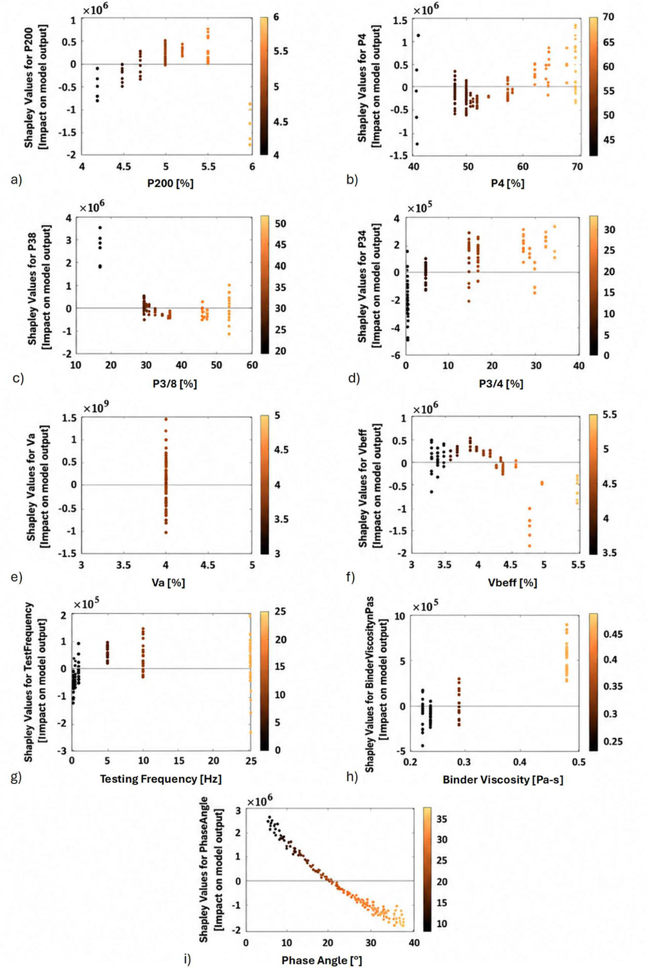
Figure 10:
SHAP dependence plots for the Cubic SVM model
Binder viscosity has a positive correlation with DM predictions and contributes to the predictions by as much as +8 x 10⁵ at the higher end of its range (approximately 0.45–0.50 Pa · s). On the other hand, Vbeff shows a non-monotonic relationship with predicted DM, with positive SHAP values when Vbeff is below 4.5% and negative, otherwise indicating that the peak model response occurs at 4.5%. The findings demonstrate the need for a balance between binder stiffness and content when employing a mix design for asphalt concrete. However, the above-mentioned thresholds should be interpreted within the experimental bounds of the data used in this study and would require experimental validation through controlled experiments.
5.4. Implications for Prediction Accuracy and Mix Design
The predictive accuracy of the data improved considerably with the use of machine learning models compared with traditional methods of analysis, as shown in Table 6 and Figure 7. With regard to both metrics (the R2 value and RMSE), the CSVM performed better than the other models. Even when compared with the next best model, the QSVM, its accuracy was 10% higher.
In addition, the better performance from SVM models compared with the Witczak model may be attributed to their ability to capture complex nonlinear relationships without predefined assumptions. Unlike the Witczak model, which is a regression-based model with high sensitivity to calibration, the CSVM performed consistently across the entire dataset, with no need for recalibration. Also, the use of explainable AI methods enhances interpretability in this context and provides useful information for data-driven mix-design optimization.
The feature importance results shown in Figure 9 and the SHAP dependency analysis results in Figure 10 provide a strong basis for determining how each parameter influences DM. The most important factor is the phase angle, which provides an important guideline for quality assurance during pavement construction. This finding suggests that the measurement and control of binder viscosity (linked with phase angle) should receive greater attention than volumetric properties when implementing performance-based design, especially for pavement designs subjected to heavy traffic loads. The next three most important factors are aggregate gradation parameters (P3/8, P200, P4), and their dependence plots provide important thresholds for design. According to these plots, coarse aggregate (P3/8) should be restricted to 45%, fine aggregate (P4) should exceed 55%, while fine particles (P200) should be maintained within the range of 5.2–5.4%. These limits would potentially maximize cohesion and stiffness in the asphalt mix by optimizing mastic properties and aggregate interlock.
The SHAP analysis of Vbeff highlights an important design pitfall wherein binder content is often increased to compensate for lower binder stiffness. This analysis provides a practical threshold in this regard, with a minimum value of 4.5%, below which there is a significant reduction in DM. However, the positive effect of higher binder stiffness cannot be neglected, and binder viscosity should be kept within 0.45–0.50 Pa·s, with a moderate binder content to maximize its contribution to DM. The test frequency and Va showed a negligible impact on the predictions, probably due to the experimental design procedure constraining these variables to a narrow range. Hence, a dedicated experimental program would be required to further investigate their impacts.
6. Conclusion
The study investigated the development and evaluation of eight different machine learning techniques to predict the DM of HMA. A comprehensive database was used in this research that included a wide range of parameters related to asphalt mixture properties, volumetric characteristics, and test conditions, which are commonly used in traditional prediction models. Results showed that the prediction performance of each model was significantly influenced by its capacity to identify nonlinear asphalt behavior. Based on the results obtained from the evaluation, it can be determined that the CSVM had the highest predictive accuracy compared to the other models tested (R2 = 0.96; RMSE = 2.22 x 10⁵ psi), followed closely by the QSVM (R2 = 0.95). In comparison, the LR model performed relatively poorly (R2 = 0.90), demonstrating the limitations of using linear approaches to describe the complex viscoelastic responses exhibited by asphalt mixtures. Although the ILR model showed improved prediction performance (R2 = 0.94) compared to the LR model, it still performed less well than all the kernel-based SVM models. Decision Trees individually produced lower prediction accuracy (R2 = 0.89). Ensemble methods were able to improve upon those results for some datasets by reducing variance, although they were unable to produce results that were better than those of the SVM models, which consistently produced accurate and generalized predictions over the full range of DM values. These comparative results are not to be generalized until sufficient trials have been done with different cross-validation and dataset split schemes.
The results obtained from the machine learning models, especially the CSVM (R2 = 0.9645), were substantially better than those typically reported for the Witczak model in the literature. This model is one of the most popular mechanistic–empirical pavement design tools. Hence, the machine learning approach shows potential as a flexible and reliable option for future pavement design, with the ability to capture the variability associated with different environments and aggregate combinations.
F Feature importance analysis indicated that the Phase Angle was the most important factor in the model (SHAP ≈ (1.05 x 10⁶)), followed closely by key gradation parameters (P3/8 and P200) and binder-related properties (Vbeff and viscosity). These findings provide an initial assessment of the factors influencing DM and demonstrate a data-driven approach for optimizing mix design. An important implication of the SHAP analysis is the potential importance of phase angle in the design of high-performance pavements, especially for heavy traffic conditions. The SHAP analysis also indicated sensitivity in model predictions to critical values of coarse and fine aggregates, with P3/8<45%, P4>55% and 5.2%<P200<5.4%. Regarding binder content and properties, the analysis also showed a significant change in their contributions to the predictions at a binder content of 4.5% and a viscosity of 0.45–0.50 Pa·s, indicating a peak model response within these ranges.
Ultimately, this study demonstrated that machine learning can improve prediction accuracy and provide a better understanding of material behavior, which may support the development of more durable and performance-oriented asphalt pavements. However, this research also has limitations, including the lack of field testing, the use of local materials and Marshall mix design procedures, and a partially crossed (unbalanced) matrix compiled from independent research projects. Therefore, the models and findings of this study, despite capturing potential mechanistic relationships between the parameters, should be considered valid within the studied domain. The limitation associated with the observation level random test split, resulting in measurements from the same mixture occurring in training and test subsets, is also acknowledged. Accordingly, the generalizability of the model and mix-design parameters derived from it should only be considered with appropriate validation. Moreover, future studies should focus on evaluating environmental factors under field conditions, incorporating a wider range of materials, using Superpave mix design procedures, and implementing a full-factorial, balanced design of experiments. External validation of the models on an independent set of mixtures, ideally from a different material source or project, is also recommended as future work.
Acknowledgement
The authors gratefully acknowledge the support provided for the experimental program. The experimental work was conducted at the laboratories of the National Institute of Transportation, National University of Sciences and Technology (NUST), whose facilities and technical assistance are sincerely appreciated.
Notes
[1] Contributed by Author's Contributions
M.A.: Conceptualization, Formal analysis, Investigation, Methodology, Software, Visualization, Writing – original draft. U.G.: Conceptualization, Methodology, Validation, Writing – original draft, Writing – review & editing. M.J.: Conceptualization, Data curation, Funding acquisition, Investigation, Project administration, Resources, Supervision, Writing – original draft, Writing – review & editing. R.I.: Conceptualization, Methodology, Validation, Writing – review & editing.