

Table 1:
Comparative assessment of predictive methods for progressive collapse analysis (adapted from Mansour et al., 2025)
| Feature [–] | DEM | FEM | AEM | Physics-Based Gaming Engines | ML |
|---|---|---|---|---|---|
| Modelling detail | High | Moderate | High | High | Low |
| Accuracy | High | High | High | Low | High |
| Computational cost | Very high | High | High | Low | Moderate |
| Ease of use | Complex | Complex | Complex | Moderate | Easy |
| Real-time capability | None | None | Moderate | High | High |
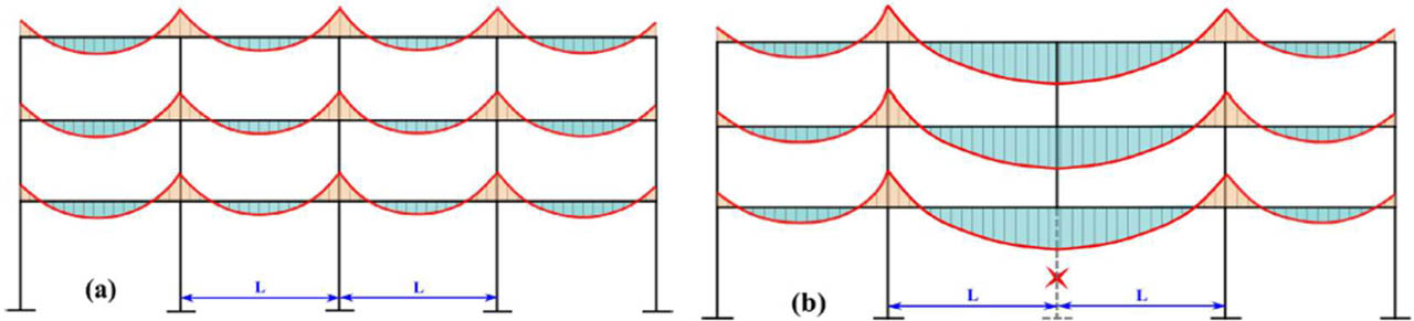
Figure 1:
Structural bending moments (a) before column removal, and (b) increase in bending moment after column removal due to span increase (reproduced from Mansour et al., 2025)
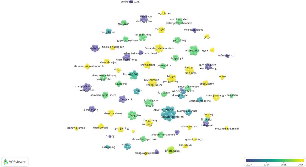
Figure 2:
VOSviewer author network map of the reviewed literature on AI-based progressive collapse and structural surrogate modelling, with nodes colored by publication year (2023–2026)
Table 2:
Summary of reviewed machine learning studies for progressive collapse and structural surrogate modelling
| Study | Structural typology | Output indicator(s) | Dataset scale [–] | Key contribution |
|---|---|---|---|---|
| Fu (2020) | Steel framed buildings | Collapse classification (fire induced) | Not reported at large scale | Feasibility of ML classification for collapse potential |
| Zhu et al. (2022) | Steel moment frames | DIF (dynamic, single indicator) | Database of pushdown analyses | ML prediction of dynamic amplification |
| Esfandiari et al. (2023) | 3D reinforced concrete frames | Collapse resistance (multi column removal) | >600 optimized frames | Self training ML on limited labelled data |
| Guo et al. (2025) | Steel frame composite floors | Collapse resistance and probability (dual) | Not directly comparable (mechanics based substructure) | Joint prediction with SHAP interpretability |
| Zhao et al. (2025) | General structural frames (static) | Displacement | >300,000 FE simulations | Ensemble averaging across six surrogate families |
| Lee et al. (2025a) | Structural and thermal response (general) | Structural/thermal response fields | Not progressive collapse specific | Identified data imbalance degradation in DNN surrogates |
| Mansour et al. (2025) (authors' prior work) | Steel moment frames | LIF (static, single indicator) | 3,990 FE models | Feasibility benchmark of ML vs FE vs DEM/AEM/gaming methods |
| Present study | Steel moment frames | LIF and DIF (joint) | 32,886 configuration–scenario records | Overfitting-aware benchmarking across 11 architectures; public deployment |
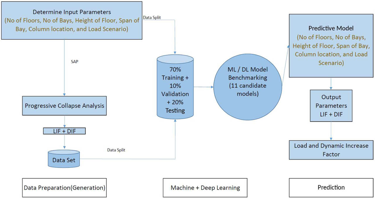
Figure 3:
Overall workflow of the proposed framework, from parametric input definition through nonlinear FE analysis, dataset partitioning, and model training, to prediction of the Load Increase Factor and Dynamic Increase Factor
Table 3:
Parametric dataset generation summary
| Stage | Count [–] | Description |
|---|---|---|
| Base building configurations | 10,962 | Factorial combination of stories, story height, span, bays, and column location |
| Configuration–scenario combinations | 32,886 | Base configurations × 3 load scenarios |
| LIF label source | – | SAP2000 nonlinear static pushdown analyses |
| DIF label source | – | SAP2000 nonlinear dynamic analyses with sudden column removal |
| Unique records in ML dataset | 32,886 | Each labelled jointly with LIF and DIF |
Table 4:
Descriptive statistics of the target variables (LIF and DIF) across the full dataset
| Target | Minimum [–] | Maximum [–] | Mean [–] |
|---|---|---|---|
| Load Increase Factor-(LIF) | 1.02 | 3.65 | 2.26 |
| Dynamic Increase Factor-(DIF) | 1.18 | 4.24 | 2.60 |
Table 5:
Definition of the three load scenarios
| Scenario | Load pattern on the main beam | Structural idealisation | Applied in | Magnitude / basis |
|---|---|---|---|---|
| 1 | Uniformly distributed load | One-way slab action | LIF (nonlinear static pushdown) and DIF (nonlinear dynamic) | Base: qDL = 3.0 kN/m2; qLL = 2.5 kN/m2; beam line load = q × tributary width. |
| 2 | Trapezoidal or triangular distributed load | Two-way slab action (tributary-area theory) | LIF (nonlinear static pushdown) and DIF (nonlinear dynamic) | Same base gravity loads; line load varies along the beam according to tributary-area geometry. |
| 3 | Concentrated load at midspan | Point load at the centre of the main beam | LIF (nonlinear static pushdown) and DIF (nonlinear dynamic) | Same base gravity load resultant as the affected beam load, represented as a midspan point load. |
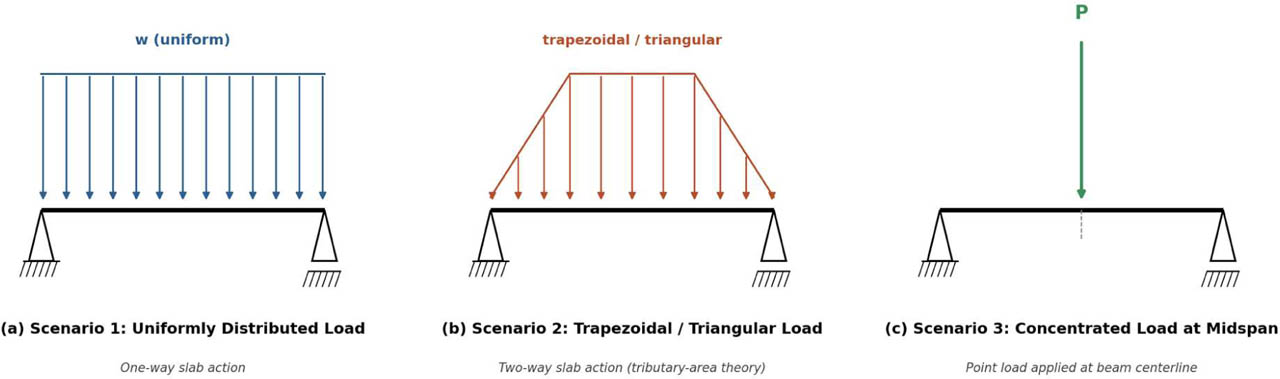
Figure 4:
Load scenarios applied to the main beam: (a) uniformly distributed load, (b) trapezoidal or triangular distributed load, and (c) concentrated load at midspan
Table 6:
Fitted standardization statistics for the four numerical input features, computed on the training partition
| Feature | Unit | Mean | Standard deviation |
|---|---|---|---|
| Number of stories | [–] | 16.05 | 8.36 |
| Story height | [m] | 4.00 | 0.81 |
| Bay span | [m] | 6.98 | 2.00 |
| Number of bays | [–] | 5.96 | 2.58 |
Table 7:
Dataset partitioning at the configuration level
| Partition | Configurations [–] | Records [–] | Proportion [%] |
|---|---|---|---|
| Training | 7,673 | 23,019 | 70 |
| Validation | 1,096 | 3,288 | 10 |
| Test | 2,193 | 6,579 | 20 |
| Total | 10,962 | 32,886 | 100 |
Table 8:
Benchmarked model architectures and hyperparameters
| Model | Family | Key hyperparameters |
|---|---|---|
| Linear regression | Classical | Ordinary least squares |
| Polynomial regression | Classical | Degree 3 |
| Random forest | Classical (ensemble) | 100 trees |
| Gradient boosting | Classical (ensemble) | 100 estimators, learning rate 0.1, maximum depth 3 |
| Support-vector regression | Classical (kernel) | RBF kernel, C = 10, ɛ = 0.1 |
| XGBoost | Classical (ensemble) | 200 estimators, learning rate 0.05, maximum depth 6 |
| LightGBM | Classical (ensemble) | 200 estimators, learning rate 0.05, 31 leaves per tree |
| DL-1 Simple | Deep learning | Fully connected, 64–32, ReLU |
| DL-2 BN+Dropout | Deep learning | Fully connected, 128–64, ReLU, batch normalisation, dropout |
| DL-3 Deep | Deep learning | Fully connected, 256–128–64, ReLU |
| DL-4 Regularised | Deep learning | Fully connected, 128–128–64, ReLU, batch normalisation, dropout |
Table 9:
Effect of the splitting strategy on test accuracy and train–validation gap. Italic: gap above 0.01
| Model | Split | Test R2 LIF [–] | Test R2 DIF [–] | Gap LIF [–] | Gap DIF [–] |
|---|---|---|---|---|---|
| Random forest | Row-level | 0.9793 | 0.9713 | 0.0189 | 0.0255 |
| Random forest | Configuration | 0.9589 | 0.9377 | 0.0391 | 0.0574 |
| LightGBM | Row-level | 0.9711 | 0.9579 | 0.0025 | 0.0019 |
| LightGBM | Configuration | 0.9664 | 0.9535 | 0.0110 | 0.0096 |
| XGBoost | Row-level | 0.9656 | 0.9529 | 0.0073 | 0.0063 |
| XGBoost | Configuration | 0.9640 | 0.9492 | 0.0132 | 0.0105 |
| Linear | Row-level | 0.9541 | 0.9405 | 0.0118 | 0.0097 |
| Linear | Configuration | 0.9542 | 0.9406 | 0.0001 | −0.0008 |
Table 10:
Grouped five-fold cross-validated train–validation gap (mean ± standard deviation). Italic: mean gap above 0.01
| Model | Gap LIF [–] | Gap DIF [–] |
|---|---|---|
| Linear | 0.0001 ± 0.0009 | 0.0001 ± 0.0021 |
| Polynomial | 0.0004 ± 0.0009 | 0.0006 ± 0.0021 |
| Gradient boosting | 0.0019 ± 0.0010 | 0.0025 ± 0.0022 |
| SVR | 0.0021 ± 0.0014 | 0.0037 ± 0.0026 |
| LightGBM | 0.0056 ± 0.0017 | 0.0085 ± 0.0033 |
| XGBoost | 0.0080 ± 0.0013 | 0.0113 ± 0.0024 |
| Random forest | 0.0374 ± 0.0021 | 0.0578 ± 0.0036 |
Table 11:
Performance of all eleven models for LIF and DIF on the configuration-level split. Bold: selected model (DL-3 Deep). Italic: train–validation gap above 0.01. Gap = train R2 − validation R2; a negative gap indicates a higher validation than training R2
| Model | Target | Train R2 [–] | Val R2 [–] | Gap [–] | Test R2 [–] | RMSE [–] | MAE [–] | MAPE [%] |
|---|---|---|---|---|---|---|---|---|
| Linear | LIF | 0.9516 | 0.9515 | 0.0001 | 0.9542 | 0.1019 | 0.0671 | 3.06 |
| Linear | DIF | 0.9373 | 0.9381 | −0.0008 | 0.9406 | 0.1335 | 0.0920 | 3.66 |
| Polynomial (deg 3) | LIF | 0.9526 | 0.9514 | 0.0012 | 0.9544 | 0.1017 | 0.0678 | 3.09 |
| Polynomial (deg 3) | DIF | 0.9383 | 0.9381 | 0.0002 | 0.9408 | 0.1333 | 0.0927 | 3.68 |
| Random forest | LIF | 0.9981 | 0.9590 | 0.0391 | 0.9589 | 0.0965 | 0.0753 | 3.39 |
| Random forest | DIF | 0.9976 | 0.9402 | 0.0574 | 0.9377 | 0.1367 | 0.1072 | 4.20 |
| Gradient boosting | LIF | 0.9549 | 0.9516 | 0.0033 | 0.9556 | 0.1003 | 0.0688 | 3.14 |
| Gradient boosting | DIF | 0.9410 | 0.9391 | 0.0019 | 0.9424 | 0.1315 | 0.0935 | 3.71 |
| SVR (RBF) | LIF | 0.9576 | 0.9513 | 0.0062 | 0.9562 | 0.0996 | 0.0683 | 3.11 |
| SVR (RBF) | DIF | 0.9432 | 0.9378 | 0.0055 | 0.9418 | 0.1322 | 0.0936 | 3.70 |
| XGBoost | LIF | 0.9715 | 0.9583 | 0.0132 | 0.9640 | 0.0903 | 0.0694 | 3.16 |
| XGBoost | DIF | 0.9572 | 0.9467 | 0.0105 | 0.9492 | 0.1235 | 0.0952 | 3.77 |
| LightGBM | LIF | 0.9733 | 0.9623 | 0.0110 | 0.9664 | 0.0873 | 0.0665 | 2.98 |
| LightGBM | DIF | 0.9607 | 0.9511 | 0.0096 | 0.9535 | 0.1182 | 0.0910 | 3.56 |
| DL-1 Simple | LIF | 0.9666 | 0.9584 | 0.0082 | 0.9608 | 0.0942 | 0.0686 | 3.09 |
| DL-1 Simple | DIF | 0.9524 | 0.9457 | 0.0066 | 0.9479 | 0.1250 | 0.0925 | 3.65 |
| DL-2 BN+Dropout | LIF | 0.9520 | 0.9486 | 0.0034 | 0.9521 | 0.1042 | 0.0726 | 3.34 |
| DL-2 BN+Dropout | DIF | 0.9362 | 0.9319 | 0.0043 | 0.9355 | 0.1392 | 0.1008 | 4.04 |
| DL-3 Deep | LIF | 0.9739 | 0.9705 | 0.0033 | 0.9714 | 0.0804 | 0.0648 | 2.90 |
| DL-3 Deep | DIF | 0.9598 | 0.9569 | 0.0029 | 0.9576 | 0.1128 | 0.0896 | 3.51 |
| DL-4 Regularised | LIF | 0.9644 | 0.9561 | 0.0083 | 0.9595 | 0.0957 | 0.0705 | 3.23 |
| DL-4 Regularised | DIF | 0.9497 | 0.9429 | 0.0068 | 0.9453 | 0.1281 | 0.0972 | 3.88 |
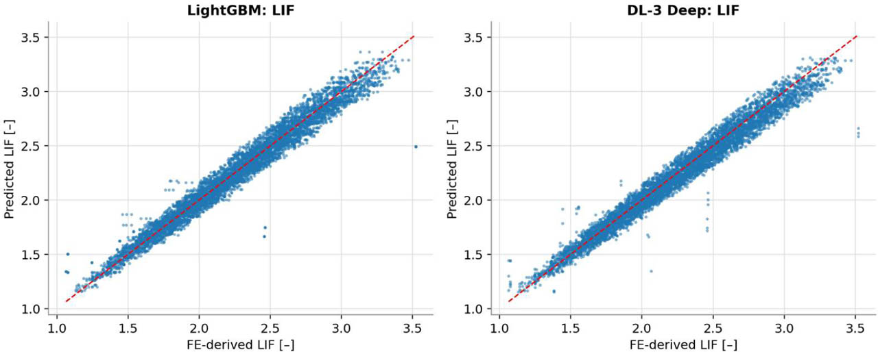
Figure 5:
Predicted versus FE-derived LIF for the selected LightGBM and DL-3 Deep models on the held-out test set
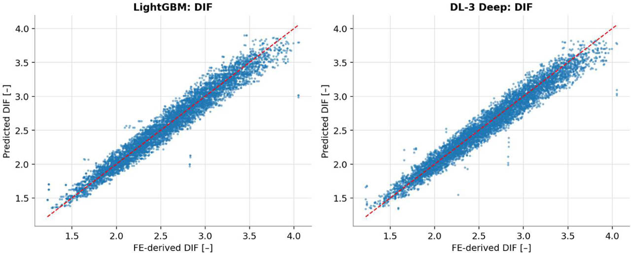
Figure 6:
Predicted versus FE-derived DIF for the selected LightGBM and DL-3 Deep models on the held-out test set
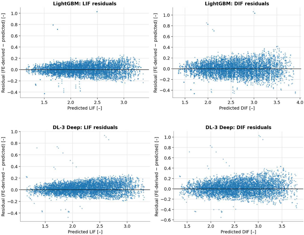
Figure 7:
Residual distributions for LIF and DIF predictions on the held-out test set, for LightGBM (top) and DL-3 Deep (bottom)
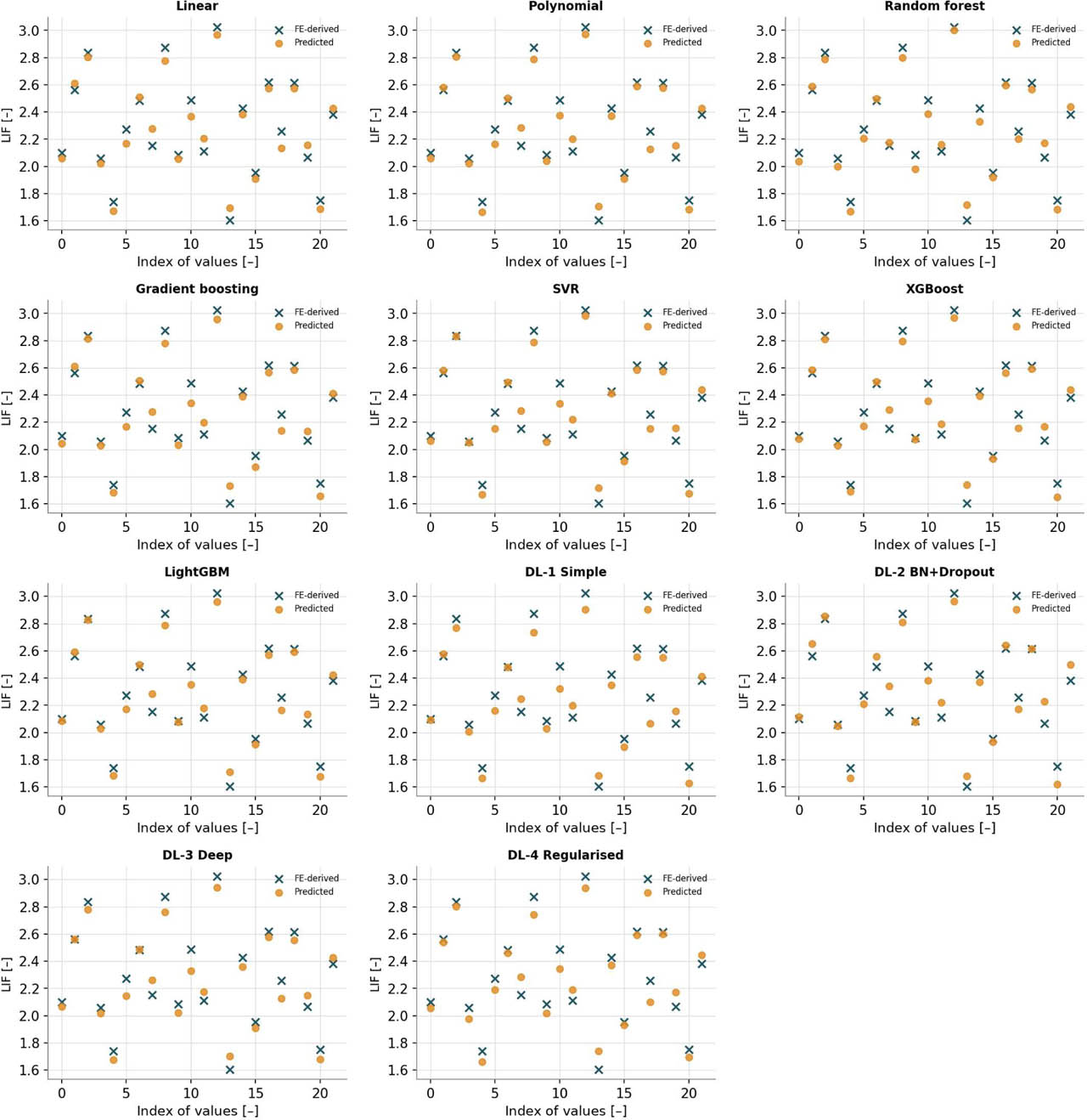
Figure 8:
Predicted versus FE-derived LIF for all eleven benchmarked models on a random subsample of 22 held-out test-set configurations
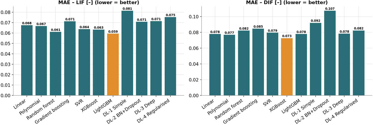
Figure 9:
Mean absolute error (MAE) for LIF and DIF across all eleven models, computed on the 22-configuration illustrative subsample
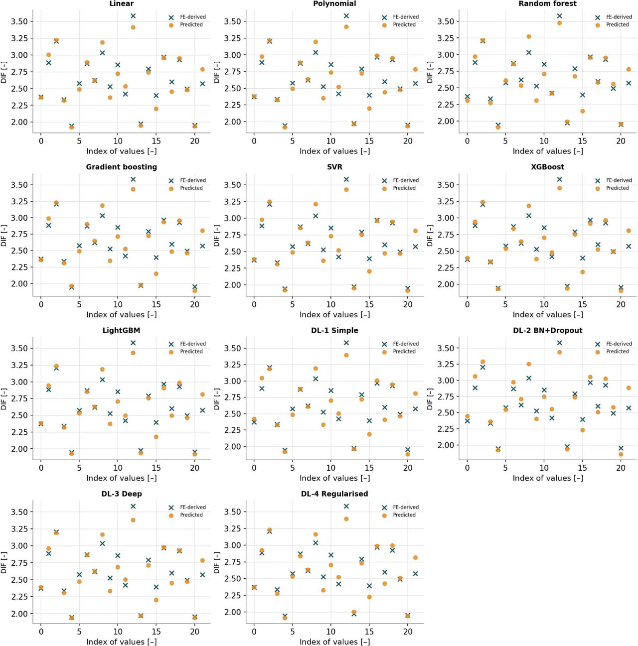
Figure 10:
Predicted versus FE-derived DIF for all eleven benchmarked models on a random subsample of 22 held-out test-set configurations
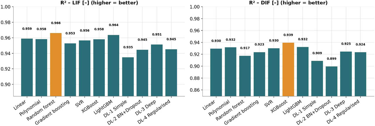
Figure 11:
Coefficient of determination (R2) for LIF and DIF across all eleven models, computed on the 22-configuration illustrative subsample
Table 12:
Model-based sensitivity of the LightGBM predictions on the test set: mean absolute SHAP value and permutation importance (drop in R2)
| Input | Mean |SHAP| LIF [–] | Mean |SHAP| DIF [–] | Permutation ΔR2 LIF [–] | Permutation ΔR2 DIF [–] |
|---|---|---|---|---|
| Number of stories | 0.373 | 0.429 | 1.607 | 1.600 |
| Bay span | 0.135 | 0.157 | 0.231 | 0.231 |
| Number of bays | 0.111 | 0.129 | 0.163 | 0.164 |
| Story height | 0.005 | 0.007 | 0.014 | 0.015 |
| Column removal location | 0.005 | 0.006 | 0.013 | 0.013 |
| Load scenario | 0.000 | 0.000 | 0.000 | 0.000 |
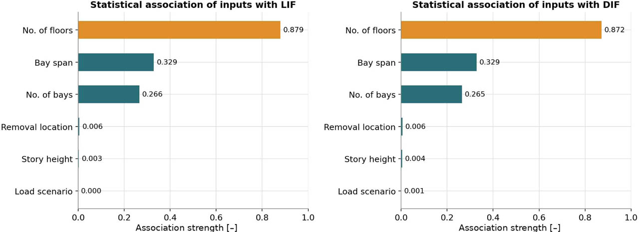
Figure 12:
Statistical association of inputs with LIF and DIF (|Pearson r| for numerical inputs; correlation ratio η for categorical inputs)
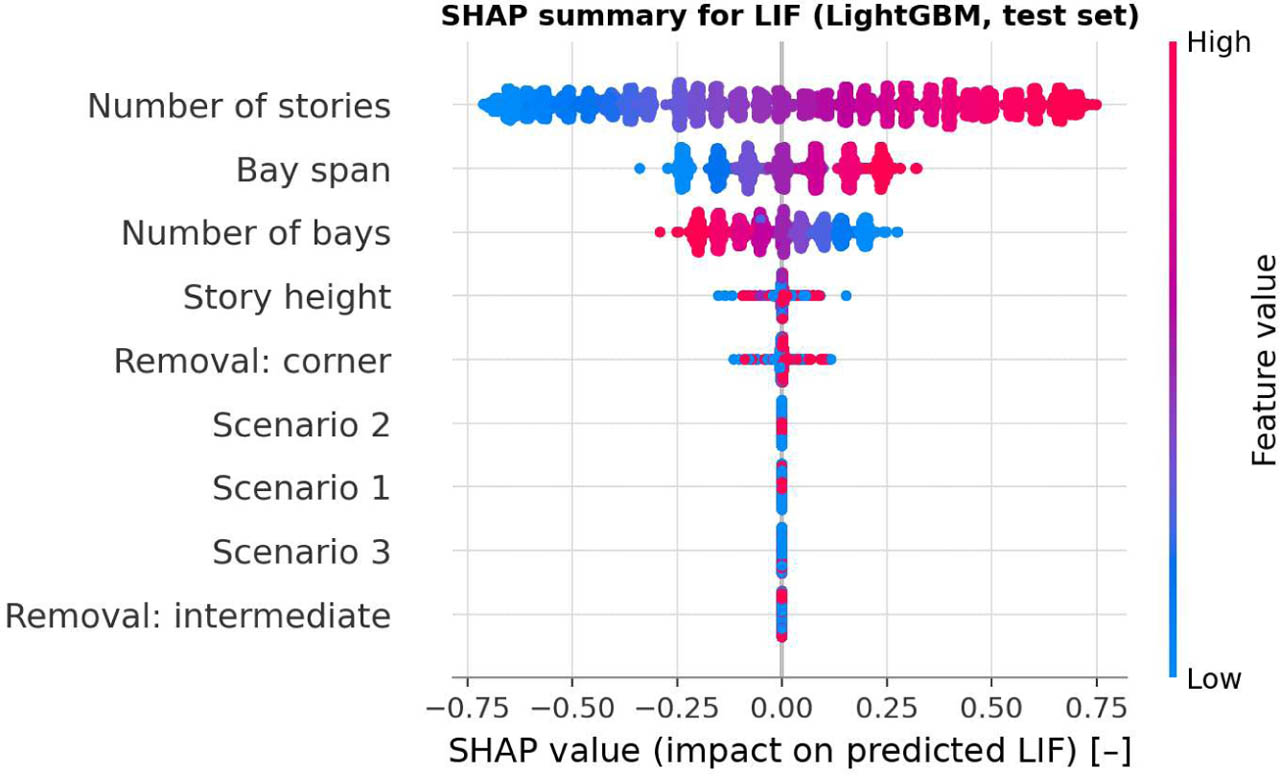
Figure 13:
SHAP summary plot for LIF (LightGBM, test set)
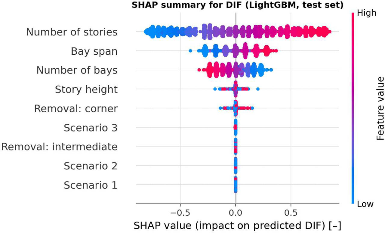
Figure 14:
SHAP summary plot for DIF (LightGBM, test set)
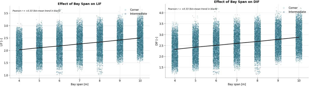
Figure 15:
Effect of bay span on LIF and DIF across the full dataset, by column-removal location
Table 13:
Comparison of FE-derived LIF and DIF with DL-3 Deep and LightGBM predictions for six held-out configurations. Δ is the percentage deviation of the prediction from the FE-derived value; S1 to S3 denote load scenarios 1 to 3
| Configuration (stories / height / span / bays / location / scenario) | FE LIF [–] | FE DIF [–] | DL-3 LIF [–] | Δ [%] | DL-3 DIF [–] | Δ [%] | LightGBM LIF Δ [%] | LightGBM DIF Δ [%] |
|---|---|---|---|---|---|---|---|---|
| 3 / 5 m / 8 m / 6 / Corner / S3 | 1.694 | 1.894 | 1.712 | +1.1 | 1.972 | +4.1 | −0.8 | +1.9 |
| 2 / 3 m / 6 m / 7 / Intermediate / S2 | 1.524 | 1.775 | 1.492 | −2.1 | 1.715 | −3.4 | +16.2 | +6.9 |
| 10 / 4 m / 9 m / 5 / Intermediate / S1 | 2.065 | 2.425 | 2.184 | +5.7 | 2.523 | +4.0 | +4.3 | +1.9 |
| 16 / 3 m / 5 m / 5 / Intermediate / S3 | 2.318 | 2.488 | 2.158 | −6.9 | 2.496 | +0.3 | −6.5 | +0.2 |
| 28 / 3 m / 9 m / 9 / Intermediate / S1 | 3.019 | 3.413 | 2.843 | −5.8 | 3.278 | −4.0 | −4.7 | −2.5 |
| 28 / 3 m / 10 m / 3 / Corner / S1 | 3.237 | 3.966 | 3.209 | −0.9 | 3.702 | −6.7 | −1.8 | −7.3 |
| Mean absolute deviation | 3.76 | 3.74 | 5.70 | 3.45 |
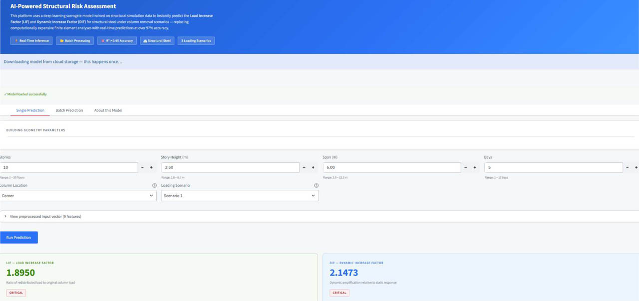
Figure 16:
Interface of the deployed web-based decision-support platform, showing the single-configuration prediction view, with input geometry, preprocessed feature vector, and classified LIF and DIF outputs
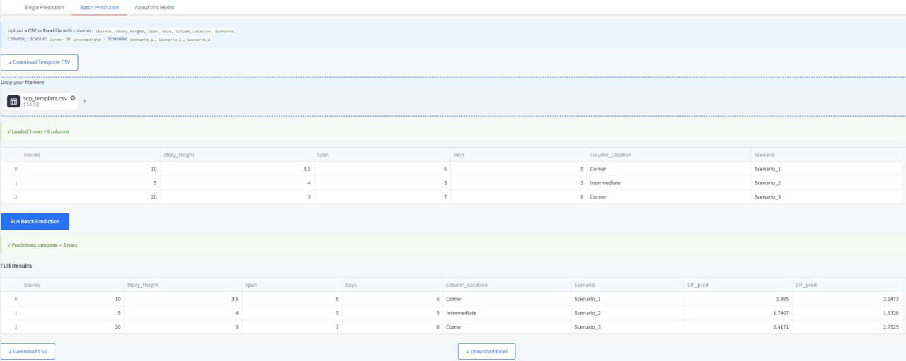
Figure 17:
Interface of the deployed web-based decision-support platform, showing the batch-prediction view with risk-band classification