

1. Introduction
Progressive collapse remains one of the most consequential failure mechanisms in multi-story steel structures, whereby the loss of a single primary member, due to blast, impact, fire, design and construction error, can trigger a chain reaction of failures disproportionate to the initial damage. Such failures can result in severe human casualties, major economic losses, and irreversible damage to landmark infrastructure. With the continuous increase in building height and structural complexity, progressive collapse assessment has become a central concern in contemporary structural design practice. Accordingly, international design guidelines and standards, including UFC 4-023-03 (Department of Defense, 2016), the GSA guidelines (General Services Administration, 2016), ASCE/SEI 7 (American Society of Civil Engineers, 2022), Eurocode EN 1991-1-7 (European Committee for Standardization, 2006), and the NBCC (National Research Council of Canada, 2020), have progressively moved toward requiring explicit evaluation of structural robustness against progressive collapse, most commonly via the alternate path method following notional column removal.
Despite this regulatory emphasis, practical implementation remains limited in everyday engineering practice. Current code-based procedures rely primarily on advanced nonlinear finite element (FE) analyses, which are computationally expensive, time consuming, and highly dependent on expert modelling skills. As a result, such analyses are typically confined to special or high-profile projects, while routine structures are often designed without systematic collapse resistance evaluation, creating a critical gap between regulatory intent and practical application.
Several studies have investigated the use of artificial intelligence (AI) and machine learning (ML) to close this gap by approximating computationally intensive progressive collapse simulations. Fu (2020) demonstrated that decision trees, k nearest neighbours, and neural networks could rapidly classify fire induced failure patterns and progressive collapse potential in steel framed buildings, achieving satisfactory prediction accuracy from a Monte Carlo generated training set. Zhu et al. (2022) trained several ML models, including k nearest neighbours, XGBoost, and a one-dimensional convolutional neural network, on a database of nonlinear pushdown analyses to predict the Dynamic Increase Factor (DIF) for steel moment frames, demonstrating reliable estimation of dynamic amplification without repeated nonlinear dynamic analysis. Esfandiari et al. (2023) applied a self-training ML algorithm to a database exceeding 600 optimized three-dimensional reinforced concrete frames to predict collapse resistance under simultaneous multi column removal scenarios. More recently, Guo et al. (2025) combined mechanics-based substructure models with five ML algorithms and SHAP based interpretability analysis to predict both the collapse resistance and probability of steel frame composite floor structures, improving transparency into the relative influence of governing design parameters.
Based on these observations, it is evident that ML based surrogate modelling has strong potential to reduce the computational burden associated with progressive collapse assessment. However, despite numerous studies confirming the feasibility of this approach, most investigations have relied on comparatively small parametric datasets, targeted a single collapse resistance indicator, or been limited to a narrow structural typology, while the joint prediction of both static (LIF) and dynamic (DIF) collapse resistance indicators, validated through a rigorous, overfitting aware model selection procedure, has received limited attention. Few studies report an explicit generalization check, such as a bound on the gap between training and validation performance, to confirm that a candidate model has learned the underlying structural relationship rather than fitting incidental noise in the training set, an issue rarely addressed explicitly in existing literature. This lack of an integrated, large scale, rigorously validated, and operationally deployable framework represents a significant research gap. Addressing this gap is essential, as practicing engineers require rapid, reliable, and generalizable tools capable of supporting collapse resistance decisions across a wide range of structural configurations without repeated recourse to specialist nonlinear FE analysis.
Motivated by this gap, the present study builds on the authors' earlier feasibility investigation, which demonstrated that ML models trained on FE generated data could predict the Load Increase Factor for multi-story steel moment frames with strong correlation to numerical benchmarks (Mansour et al., 2025). This study advances the state of the art by shifting the focus from single-indicator feasibility demonstration to a fully validated, deployable assessment framework. The specific novelty of this work is threefold: (1) the development of a large scale parametric database, generated through a factorial study spanning five geometric and configurational parameters and three load scenarios, approximately eight times larger than comparable prior datasets; (2) the implementation of an overfitting aware model selection procedure, ensuring that reported accuracy reflects genuine generalization on unseen configurations rather than a spuriously high validation score; and (3) the identification and validation of accurate surrogate models that predict both collapse-resistance indicators directly from frame geometry and loading, closing the gap between numerical feasibility and practical engineering use. To achieve these objectives, the study adopts a multistage computational framework integrating nonlinear FE data generation, systematic benchmarking of machine learning and deep learning architectures, and an overfitting-aware model selection procedure. Framework predictions are directly compared to benchmark nonlinear FE simulation results for six held-out configurations spanning the validated domain. The scope of the study is limited to multi-story steel moment frames under column removal scenarios, and the discussion explicitly distinguishes between the parameter ranges represented in the training data and the broader input ranges exposed through the deployed interface, to clarify where predictions constitute reliable interpolation versus unvalidated extrapolation.
2. Related Work
2.1. Progressive Collapse Prediction
Progressive collapse prediction, in its broadest sense, refers to the assessment of whether the loss of a primary structural element leads to failure confined to the local region or propagates into disproportionate failure of the surrounding system. This assessment problem sits at the core of structural robustness design and has been formalized through the alternate path method, in which a column is notionally removed and the resulting redistribution of load through the remaining structure is evaluated against the capacity of adjacent members and connections. The governing indicators of this assessment, the Load Increase Factor (LIF) and the Dynamic Increase Factor (DIF), quantify respectively the static load redistribution demand and the dynamic amplification associated with the sudden, rather than gradual, nature of column loss. Predicting these indicators reliably and efficiently, for an arbitrary building configuration, is the underlying prediction problem that both traditional analytical methods and, more recently, machine learning based approaches attempt to solve. The progressive collapse problem and its regulatory background have been reviewed extensively (Wang et al., 2014; Byfield et al., 2014; Abdelwahed, 2019; Kiakojouri et al., 2020; Elkady et al., 2024), together with strengthening and retrofitting techniques intended to mitigate it (Kiakojouri et al., 2022) and the behaviour of steel high-rise buildings exposed to fire (Jiang and Li, 2018).
International design guidelines, including UFC 4-023-03 (Department of Defense, 2016), the GSA guidelines (General Services Administration, 2016), ASCE/SEI 7 (American Society of Civil Engineers, 2022), Eurocode EN 1991-1-7 (European Committee for Standardization, 2006), and the NBCC (National Research Council of Canada, 2020), require this prediction to be made explicitly for structures falling within their scope of applicability, rather than relying on prescriptive detailing rules alone. The GSA guidelines typically recommend a load multiplier of 2.0 for progressive collapse load combinations in static procedures, a factor intended to account jointly for inertial and nonlinear effects (Mansour et al., 2025). It is important to note that this Load Increase Factor should not be confused with the dynamic increase factors used separately in nonlinear dynamic analysis for blast loading, a distinction that is often a source of confusion in practice and one the present study maintains throughout. However, as discussed in Section 1, the computational cost of generating this prediction through conventional means restricts its routine use, motivating the search for faster prediction methods, which forms the central theme of the remainder of this section.
2.2. Methods for Prediction of Progressive Collapse
Progressive collapse prediction has historically relied on a range of computational methods, each carrying distinct trade-offs between modelling fidelity, computational cost, and practical usability. The authors' earlier work (Mansour et al., 2025) directly compared five such approaches, and that comparison is summarized here as it frames the motivation for the data-driven framework developed in the present study.
The Discrete Element Method (DEM) is highly effective for modelling discontinuous systems, capturing detailed fracture and separation behaviour at the element level, but its high computational cost limits its practicality for large-scale multi-storey structures. The Finite Element Method (FEM) offers high accuracy for continuous systems and remains the industry standard for progressive collapse assessment, yet it demands significant computational resources and specialist modelling expertise. The Applied Element Method (AEM) bridges the gap between FEM and DEM, permitting both continuum and discontinuum analysis within a single framework, which makes it well suited to structures undergoing large deformations and element separation during collapse. Physics-Based Gaming Engines represent a fourth category, having gained traction for their ability to simulate structural behaviour in real time with user-friendly, visually intuitive interfaces; however, these tools generally lack the numerical precision required for detailed structural analysis, since they are optimized for rendering speed and visualization rather than engineering accuracy. Table 1 summarizes this comparison, adapted from the authors' earlier study.
Table 1:
Comparative assessment of predictive methods for progressive collapse analysis (adapted from Mansour et al., 2025)
| Feature [–] | DEM | FEM | AEM | Physics-Based Gaming Engines | ML |
|---|---|---|---|---|---|
| Modelling detail | High | Moderate | High | High | Low |
| Accuracy | High | High | High | Low | High |
| Computational cost | Very high | High | High | Low | Moderate |
| Ease of use | Complex | Complex | Complex | Moderate | Easy |
| Real-time capability | None | None | Moderate | High | High |
This comparison illustrates the central trade-off motivating the present study. DEM, FEM, and AEM offer high modelling detail and accuracy but at very high computational cost and with limited real-time capability, while physics-based gaming engines offer real-time performance at the expense of engineering-grade accuracy. Machine learning occupies a distinct position, combining high accuracy, once trained, with low computational cost per prediction and near real-time capability, at the cost of reduced granularity in modelling detail relative to a full FE solution. It is this specific combination that positions ML as a practical middle ground for routine progressive collapse assessment, and that motivates its further development in the present study.
Beyond these five approaches, further analytical and numerical studies have addressed progressive collapse under sudden column removal. They include investigations of the column removal time and modelling approach (Stephen et al., 2019), of modal pushdown procedures for steel frames (Ferraioli, 2019), of steel structures with moment resisting frames (Mohamed and Khattab, 2019), of tall steel composite buildings (Rahnavard et al., 2018), of braced steel frames (Saberi et al., 2021; Salimi and Bondarabadi, 2021) and of the dynamic behaviour of steel frames during progressive collapse (Xie et al., 2021), together with an analytical methodology for the dynamic amplification factor (Tsai, 2010). Reinforced concrete and hybrid structures have been studied in the same way (Al-Salloum et al., 2017; Chen et al., 2018; Elshaer et al., 2017; Gowtham et al., 2018; Mourid et al., 2020). Stochastic and probabilistic frameworks (Le and Xue, 2014; Xue and Le, 2016; Javidan et al., 2018), earthquake-induced loss assessment of steel moment frames (Hwang and Lignos, 2017), the quantification of robustness (Voulpiotis et al., 2022) and the optimum design of steel frames against progressive collapse (Tayfur and Daloglu, 2024) complete this body of work. Most of these approaches rely on repeated structural analyses, which is the cost that the surrogate models studied here aim to remove.
Following the empirical formulation of Mashhadi and Saffari (2016), which was also adopted in the authors' earlier study (Mansour et al., 2025), the DAF is expressed as:
Where:DAF — dynamic amplification factor,
ζ— damping ratio,
θp — plastic rotation,
θyiels — yield rotation.
This methodology offers several advantages: it simplifies the analysis process by reducing reliance on complex dynamic simulations, it provides a computationally efficient way to estimate maximum dynamic response, and grounding the DAF in empirical formulas developed from experimental and theoretical research enhances its reliability. This approach is particularly useful for steel structures, where ductility and damping play a significant role in determining structural response under extreme loads. Figure 1 illustrates the structural bending moment redistribution before and after column removal that underlies this response prediction concept.
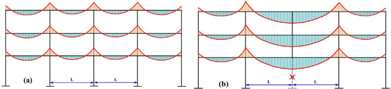
Figure 1:
Structural bending moments (a) before column removal, and (b) increase in bending moment after column removal due to span increase (reproduced from Mansour et al., 2025)
Despite its computational efficiency, the DAF approach remains an empirical approximation calibrated against a limited range of structural configurations, and its accuracy degrades outside that calibration range, a limitation shared with the broader class of empirical and semi-analytical methods reviewed here. It is this gap, between the high fidelity but high cost of DEM, FEM, and AEM, and the narrow calibration range of empirical DAF-type formulas, that machine learning based surrogate modelling has increasingly sought to close, as reviewed in the following section
2.3. Machine Learning in Structural and Progressive Collapse Prediction
Data-driven surrogate modelling has increasingly been adopted across structural engineering as a means of replacing repeated, computationally expensive finite element analyses with fast, trained approximations. Within the specific context of progressive collapse, the earliest efforts focused on demonstrating feasibility on modest datasets before more recent work has pushed toward larger databases, richer output sets, and greater methodological rigour. To characterize the scope and recency of this field before reviewing individual studies in detail, a bibliometric author network analysis was performed on the relevant literature using VOSviewer. Figure 2 presents the resulting network map, with node color indicating publication recency from 2023 to 2026 and node size reflecting relative publication or co-authorship weight within the mapped corpus.
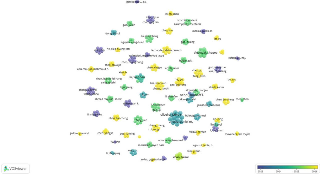
Figure 2:
VOSviewer author network map of the reviewed literature on AI-based progressive collapse and structural surrogate modelling, with nodes colored by publication year (2023–2026)
The map shows a densely populated and rapidly growing research community, organized into loosely connected clusters of co-publishing authors rather than a single dominant group, consistent with a field still in an active, decentralized growth phase rather than one consolidated around a small number of established research groups. The marked concentration of yellow and green toned, more recent nodes across the map, rather than a shift confined to one region of it, supports the trajectory noted throughout this section: progressive collapse prediction via machine learning is not a mature, settled subfield but one where the majority of contributing authors have published within the last one to two years. This recency distribution reinforces the positioning of the present study, that it sits at the leading edge of an actively developing area, and it also explains why the narrative review that follows draws primarily on studies published in 2023 or later, since these represent the dense, recent core of the network shown in Figure 2 rather than a sparse historical tail.
Fu (2020) provided one of the first demonstrations that machine learning could support progressive collapse assessment, applying decision trees, k nearest neighbours, and neural networks to classify fire induced failure patterns in steel framed buildings. The training data were generated through Monte Carlo sampling, and the study established that classification style outputs, such as collapse or no collapse, could be predicted with satisfactory accuracy without repeated nonlinear analysis. However, the work was limited to a classification framing rather than a continuous prediction of collapse resistance indicators, and the dataset size was not reported at a scale comparable to the parametric studies that followed. As an earlier, 2020-dated contribution, this study predates the dense cluster of activity visible in Figure 2 and represents part of the field's initial foundation rather than its current growth phase.
Zhu et al. (2022) advanced this line of work by predicting a continuous structural response, the Dynamic Increase Factor, using k nearest neighbours, XGBoost, and a one dimensional convolutional neural network trained on a database of nonlinear pushdown analyses for steel moment frames. Their results demonstrated that dynamic amplification effects, which normally require a separate nonlinear dynamic analysis beyond the static pushdown case, could be reliably approximated by a trained surrogate. This represented an important step beyond classification, but the study addressed only the dynamic response indicator and did not extend to the static Load Increase Factor within the same framework.
Esfandiari et al. (2023) examined a different structural typology, applying a self training machine learning algorithm to a database exceeding 600 optimized three dimensional reinforced concrete frames in order to predict collapse resistance under simultaneous multi column removal scenarios. This work highlighted the value of self training approaches in settings where labelled data are comparatively expensive to generate, and it broadened the scope of progressive collapse machine learning research beyond steel structures. Nonetheless, the dataset size remained an order of magnitude smaller than what large scale parametric FE generation can provide, and the semi supervised nature of the approach introduces additional uncertainty regarding the reliability of pseudo labelled samples. This study falls within the 2023 entry point of the network in Figure 2, marking the beginning of the field's more active recent phase.
More recently, Guo et al. (2025) combined mechanics based substructure models with five machine learning algorithms and SHAP based interpretability analysis to jointly predict the collapse resistance and the collapse probability of steel frame composite floor structures. This study is notable for two reasons directly relevant to the present work: it addressed more than one output indicator within a single framework, and it introduced interpretability analysis to clarify which geometric and loading parameters most strongly influence the predicted response. The interpretability contribution is valuable for engineering trust in the model, though the study's scope was specific to composite floor systems rather than steel moment frames under column removal.
Machine learning has also been applied to progressive collapse of other structural forms. Esfandiari and Urgessa (2020) combined structural optimization and machine learning for the progressive collapse design of reinforced concrete frames, Gan et al. (2023) predicted the progressive collapse resistance of reinforced concrete frames with a deep and cross network model, Liu et al. (2024b) developed machine learning models for the progressive collapse resistance of truss string structures, and Wang et al. (2023) combined machine learning with a physics engine for the rapid visual simulation of progressive collapse in regular reinforced concrete frames. Wang et al. (2025) further assessed progressive collapse regions of reinforced concrete frame structures using graph convolutional networks. These studies confirm the growing use of data-driven models for collapse assessment, but they address reinforced concrete or special structural forms rather than steel moment frames under column removal.
Beyond the progressive collapse literature specifically, recent work on structural surrogate modelling more broadly reinforces two methodological themes that motivate the present framework. Zhao et al. (2025) proposed a Jackknife Model Averaging ensemble that combined six surrogate models, including polynomial response surfaces, support vector regression, and gradient boosted tree methods, evaluated on a static analysis dataset exceeding 300,000 finite element simulations. Their results showed that ensemble averaging consistently outperformed any individual surrogate in terms of error and calibration, underscoring the value of benchmarking multiple model families rather than committing to a single algorithm a priori, an approach mirrored in the present study's comparison of seven machine learning algorithms and four deep learning architectures. Separately, Lee et al. (2025a) examined the problem of data imbalance in deep learning based surrogate models for structural and thermal response prediction, showing that when low magnitude responses dominate a training set, deep neural networks can suffer degraded performance in the underrepresented, higher response regions that are often the most safety critical. This finding is directly relevant to progressive collapse surrogate modelling, where duplicate or densely clustered records in a parametrically generated dataset can distort the effective distribution of training samples in a similar way, reinforcing the importance of the duplicate screening procedure adopted in the present study. Both of these 2025-dated contributions sit within the yellow, most recent band of nodes in Figure 2.
Machine learning has been applied across structural engineering more widely, as summarised in several reviews (Salehi and Burgueño, 2018; Thai, 2022; Marzouk et al., 2024; Kraus and Drass, 2020). Applications include vibration-based and image-based damage detection and assessment (Avci et al., 2021; Daneshvar and Sarmadi, 2022; Chen et al., 2023), long-term structural health monitoring of caisson quay walls (Lee et al., 2025b), data augmentation for structural health monitoring and electromechanical admittance data (Ai and Zhang, 2023; Zheng et al., 2025), damage levels of bridges in vehicular collision fires (Moradi et al., 2023), blast loading prediction (Li et al., 2023; Li et al., 2025), the behaviour and failure modes of connections and members (Cabrera et al., 2023; Kabir et al., 2021; Xu et al., 2025), seismic demand and collapse (Hwang et al., 2021; Sediek et al., 2022), the sensitivity of steel frames with imbalanced, high-dimensional data (Koh and Blum, 2022), the blast response of reinforced concrete slabs (Zhou et al., 2024), the strength of slabs (Alateyat et al., 2024; Albostami et al., 2025; Liu et al., 2024a), prestressing force in bridges (Calò et al., 2025) and the optimisation of braced structures (Zhang et al., 2025). These works show that data-driven surrogates are established tools in structural engineering, and the present study applies the same idea to the joint prediction of the LIF and DIF of steel frames.
Table 2:
Summary of reviewed machine learning studies for progressive collapse and structural surrogate modelling
| Study | Structural typology | Output indicator(s) | Dataset scale [–] | Key contribution |
|---|---|---|---|---|
| Fu (2020) | Steel framed buildings | Collapse classification (fire induced) | Not reported at large scale | Feasibility of ML classification for collapse potential |
| Zhu et al. (2022) | Steel moment frames | DIF (dynamic, single indicator) | Database of pushdown analyses | ML prediction of dynamic amplification |
| Esfandiari et al. (2023) | 3D reinforced concrete frames | Collapse resistance (multi column removal) | >600 optimized frames | Self training ML on limited labelled data |
| Guo et al. (2025) | Steel frame composite floors | Collapse resistance and probability (dual) | Not directly comparable (mechanics based substructure) | Joint prediction with SHAP interpretability |
| Zhao et al. (2025) | General structural frames (static) | Displacement | >300,000 FE simulations | Ensemble averaging across six surrogate families |
| Lee et al. (2025a) | Structural and thermal response (general) | Structural/thermal response fields | Not progressive collapse specific | Identified data imbalance degradation in DNN surrogates |
| Mansour et al. (2025) (authors' prior work) | Steel moment frames | LIF (static, single indicator) | 3,990 FE models | Feasibility benchmark of ML vs FE vs DEM/AEM/gaming methods |
| Present study | Steel moment frames | LIF and DIF (joint) | 32,886 configuration–scenario records | Overfitting-aware benchmarking across 11 architectures; public deployment |
Taken together, this body of work, and its concentration in the recent, densely connected portion of the author network shown in Figure 2, establishes three consistent conclusions. First, machine learning and deep learning surrogates can approximate nonlinear structural responses relevant to progressive collapse with strong accuracy, consistently reported in the range of 0.93 to above 0.99 in terms of the coefficient of determination across the studies reviewed. Second, the trend in the field has moved from single indicator, classification style outputs toward joint prediction of multiple continuous response quantities, paralleling the broader movement in structural surrogate modelling toward multi output and interpretable frameworks. Third, and most significantly for the present study, few investigations have paired a large scale, systematically generated parametric dataset with a model selection procedure that explicitly guards against overfitting, and fewer still have carried a validated surrogate model through to a publicly deployable engineering tool. The present study, building on the authors' own earlier feasibility work (Mansour et al., 2025), addresses this combination directly: a factorial parametric database approximately eight times larger than comparable prior studies, a benchmarking procedure across eleven candidate architectures selected on an overfitting aware criterion, and deployment of the resulting model as an interactive, web-based decision support platform.
3. Methodology
3.1. Prediction Task and Dataset Formulation
Figure 3 presents the overall workflow adopted in this study, linking the geometric and categorical input parameters to a validated nonlinear FE analysis campaign, a partitioned and preprocessed dataset, and a trained predictive model whose outputs are the two collapse-resistance indicators of interest.
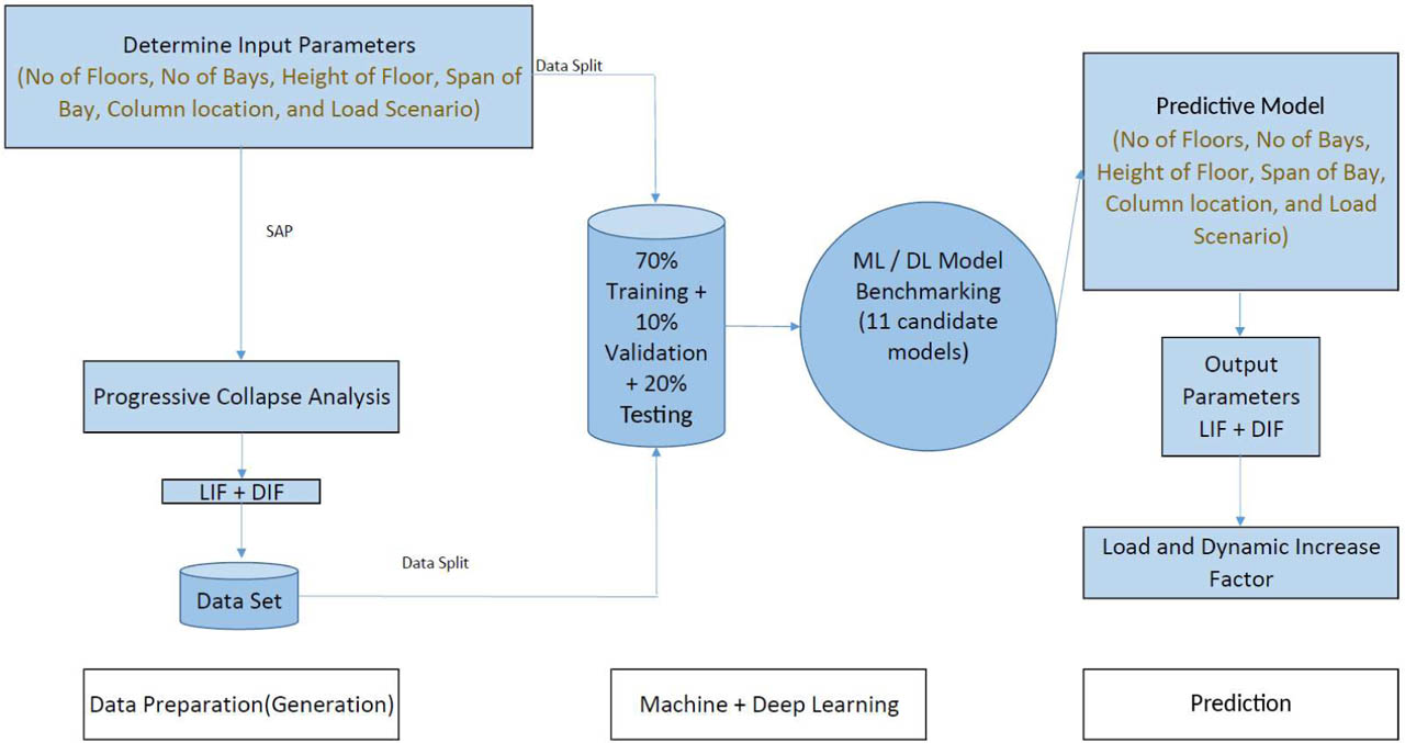
Figure 3:
Overall workflow of the proposed framework, from parametric input definition through nonlinear FE analysis, dataset partitioning, and model training, to prediction of the Load Increase Factor and Dynamic Increase Factor
The progressive collapse assessment problem addressed in this study is formulated as a supervised multi-output regression task. Given a compact description of a steel moment-frame configuration, the framework is required to simultaneously predict two continuous target quantities, the Load Increase Factor (LIF) and the Dynamic Increase Factor (DIF), without recourse to repeated nonlinear finite element (FE) analysis. Each record in the underlying database is described by six input parameters: four numerical geometric quantities, namely the number of stories, the story height [m], the bay span [m], and the number of bays, together with two categorical parameters, the column removal location and the load scenario. Each record is labelled with the LIF and DIF values obtained from the nonlinear FE analyses described in Section 3.2.
A deliberate modelling decision was made to exclude the base static factors from the set of input features, even though these quantities are available at the time of FE data generation. Including them would allow the surrogate model to infer the target factors from quantities that already partially encode the answer, producing an artificially inflated measure of predictive skill that would not transfer to a genuine design scenario, in which an engineer specifies only the geometric and loading configuration of the frame and requires the collapse-resistance indicators as an output, not an input. The surrogate is therefore required to learn the mapping from geometry and loading alone to LIF and DIF, mirroring the information available to a designer at the point the prediction is needed.
3.2. Parametric Dataset Generation
The database underlying this study was generated through a structured parametric study rather than random or opportunistic sampling. Five parameters were systematically varied to define the space of building configurations considered: the number of stories, ranging from 2 to 30 floors; the story height, taking discrete values of 3, 4, or 5 m; the in-plan bay span, ranging from 4 to 10 m; the number of bays, ranging from 2 to 10; and the column removal location, considered at either an intermediate or a corner position. All models shared a fixed out-of-plane bay spacing of 6.0 m (three bays), a dead load of 300 kg/m2, and a live load of 250 kg/m2, so that the parametric variation isolates the effect of geometry and column removal location rather than confounding it with variation in loading intensity. This factorial combination of parameters produced 10,962 unique base building configurations. All bays within a frame share a single span, with a fixed out-of-plane bay spacing of 6.0 m; frames with unequal spans are outside the validated domain and are left for future work.
The database contains 10,962 base building configurations and three defined load-scenario records for each configuration, giving 32,886 configuration–scenario records. Each record is jointly labelled with an LIF and a DIF value from the corresponding FE dataset.
Table 3:
Parametric dataset generation summary
| Stage | Count [–] | Description |
|---|---|---|
| Base building configurations | 10,962 | Factorial combination of stories, story height, span, bays, and column location |
| Configuration–scenario combinations | 32,886 | Base configurations × 3 load scenarios |
| LIF label source | – | SAP2000 nonlinear static pushdown analyses |
| DIF label source | – | SAP2000 nonlinear dynamic analyses with sudden column removal |
| Unique records in ML dataset | 32,886 | Each labelled jointly with LIF and DIF |
Table 4:
Descriptive statistics of the target variables (LIF and DIF) across the full dataset
| Target | Minimum [–] | Maximum [–] | Mean [–] |
|---|---|---|---|
| Load Increase Factor-(LIF) | 1.02 | 3.65 | 2.26 |
| Dynamic Increase Factor-(DIF) | 1.18 | 4.24 | 2.60 |
LIF and DIF are strongly co-varying, moving in the same direction in 98.6% of records, consistent with the expectation that configurations demanding greater static load redistribution also tend to exhibit greater dynamic amplification. This correlation is a further motivation for the joint, rather than independent, prediction of LIF and DIF adopted in Section 3.1
3.2.1. Finite Element Modelling
All analyses were carried out in SAP2000 within an automated parametric workflow. The parameters of the FE models are reported below in three groups, so that the reader can distinguish what is verified from the model files that are still available, what is stated from the authors' records of the study, and what is reconstructed following the applicable guideline practice because the original analysis-case log of the batch is not available.
Verified from the available SAP2000 model files: the software version (SAP2000 version 25), structural steel S355 according to EN 10025-2 and Egyptian code of practice, European wide-flange HE sections (the HEA series is used in the dataset), and the load patterns for dead load, superimposed dead load and live load.
Stated from the authors' records of the study: three-dimensional steel moment-resisting frames with an out-of-plane arrangement of three bays at 6.0 m; a dead load of 300 kg/m2 and a live load of 250 kg/m2; member sections selected for each configuration in a design stage and upsized where the force-controlled progressive collapse criterion was not satisfied, so that section sizes grow with the number of stories; and LIF obtained from a nonlinear static pushdown analysis and DIF from a nonlinear dynamic analysis with sudden column removal, extracted following the GSA alternate path framework (General Services Administration, 2016).
Settings follow GSA alternate-path, UFC 4-023-03 and ASCE 41 practice: gravity load DL + 0.25LL for the nonlinear dynamic analysis and 2.0(DL + 0.25LL) for the nonlinear static analysis; concentrated plastic hinges (M3 in beams, P-M2-M3 in columns) with ASCE 41 and UFC 4-023-03 acceptance criteria; geometric nonlinearity (P-Δ and large displacements) in both analyses; rigid beam-column connections and fixed column bases; column removal over a time not exceeding one tenth of the period of the vertical mode of the affected bay; a damping formulation and integration time step sufficiently small to resolve the column-removal event and obtain a numerically stable response; and the standard SAP2000 convergence-control settings.
3.2.2. Load Scenarios
Three load scenarios define how the gravity load (300 kg/m2 dead load and 250 kg/m2 live load, i.e. approximately 3.0 and 2.5kN/m2) is applied to the frame (Table 5 and Figure 4). Scenario 1 applies a uniformly distributed beam load representing one-way slab action. Scenario 2 applies a trapezoidal or triangular distribution derived from tributary-area theory, representing two-way slab action. Scenario 3 applies a concentrated load at the midspan of the main beam. The three patterns are defined for both the LIF and the DIF analyses.
Table 5:
Definition of the three load scenarios
| Scenario | Load pattern on the main beam | Structural idealisation | Applied in | Magnitude / basis |
|---|---|---|---|---|
| 1 | Uniformly distributed load | One-way slab action | LIF (nonlinear static pushdown) and DIF (nonlinear dynamic) | Base: qDL = 3.0 kN/m2; qLL = 2.5 kN/m2; beam line load = q × tributary width. |
| 2 | Trapezoidal or triangular distributed load | Two-way slab action (tributary-area theory) | LIF (nonlinear static pushdown) and DIF (nonlinear dynamic) | Same base gravity loads; line load varies along the beam according to tributary-area geometry. |
| 3 | Concentrated load at midspan | Point load at the centre of the main beam | LIF (nonlinear static pushdown) and DIF (nonlinear dynamic) | Same base gravity load resultant as the affected beam load, represented as a midspan point load. |
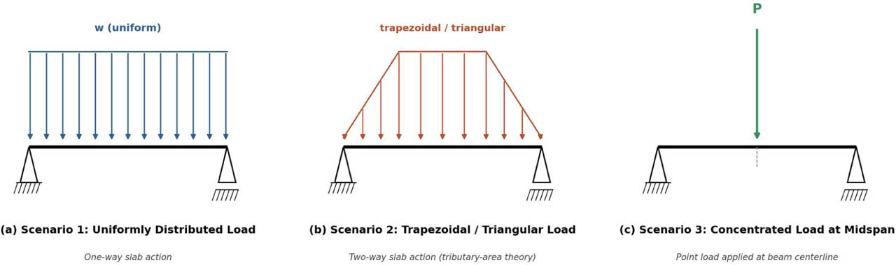
Figure 4:
Load scenarios applied to the main beam: (a) uniformly distributed load, (b) trapezoidal or triangular distributed load, and (c) concentrated load at midspan
In the dataset, the three load scenarios change LIF and DIF by less than ±3% relative to the base value of the same configuration, which is below the resolution of the surrogate models. The load scenario is retained as an input so that the deployed platform covers all three load patterns, but the models should not be used to discriminate between them.
3.3. Feature Preprocessing
All preprocessing operations were fitted exclusively on the training partition and subsequently applied, without refitting, to the validation and test partitions. This sequencing is essential to prevent information leakage: had the preprocessing statistics been computed across the full dataset before partitioning, information about the distribution of the validation and test sets would have leaked into the transformation applied to the training data, inflating the apparent generalization performance of the resulting models. The four numerical features, number of stories, story height, bay span, and number of bays, were median imputed for any missing values and subsequently standardized to zero mean and unit variance. Table 6 reports the fitted training set statistics used for this standardization.
Table 6:
Fitted standardization statistics for the four numerical input features, computed on the training partition
| Feature | Unit | Mean | Standard deviation |
|---|---|---|---|
| Number of stories | [–] | 16.05 | 8.36 |
| Story height | [m] | 4.00 | 0.81 |
| Bay span | [m] | 6.98 | 2.00 |
| Number of bays | [–] | 5.96 | 2.58 |
Standardization was performed according to Equation (2):
Where:z- standardized feature value,
x - raw feature value,
μ – training-set mean of the feature,
σ – training-set standard deviation of the feature.
This transformation ensures that features measured on different numeric scales, for example story height in the range of a few meters against number of stories in the range of tens of floors, contribute to model training on an equal footing, rather than being implicitly weighted by the magnitude of their raw units. The two categorical features, column removal location and load scenario, were most-frequent-imputed for any missing values and one-hot encoded. The column removal location was encoded into two binary columns, and the load scenario into three binary columns, giving a total model input dimension of nine features after preprocessing.
3.4. Training, Validation, and Test Partitioning
Duplicate records were removed before partitioning, leaving 32,886 unique configuration–scenario records. Each of the 10,962 base configurations appears three times, once per load scenario, and these three records differ only in the load scenario. A row-level split would therefore place near-identical siblings of a test record in the training set. The partition was consequently made at the configuration level: the 10,962 configurations were randomly assigned (random seed 42) to training, validation and test groups of 70%, 10% and 20%, and all three scenario records of a configuration were assigned to the same partition. Zero overlap of configurations between the partitions was verified explicitly. Table 7 summarizes the resulting partition sizes.
Table 7:
Dataset partitioning at the configuration level
| Partition | Configurations [–] | Records [–] | Proportion [%] |
|---|---|---|---|
| Training | 7,673 | 23,019 | 70 |
| Validation | 1,096 | 3,288 | 10 |
| Test | 2,193 | 6,579 | 20 |
| Total | 10,962 | 32,886 | 100 |
The validation partition is used exclusively for model selection, including the overfitting-aware criterion described in Section 3.6, and is never used to update model parameters directly. The test partition is held out entirely from both training and model selection and is accessed only once, to report the final performance of the selected models, as presented in Section 4.
3.5. Benchmarked Models
Eleven candidate architectures were benchmarked under identical preprocessing and partitioning conditions, comprising seven classical machine learning algorithms and four feed-forward deep neural networks. Table 8 lists the full set of candidates together with their key hyperparameters.
Table 8:
Benchmarked model architectures and hyperparameters
| Model | Family | Key hyperparameters |
|---|---|---|
| Linear regression | Classical | Ordinary least squares |
| Polynomial regression | Classical | Degree 3 |
| Random forest | Classical (ensemble) | 100 trees |
| Gradient boosting | Classical (ensemble) | 100 estimators, learning rate 0.1, maximum depth 3 |
| Support-vector regression | Classical (kernel) | RBF kernel, C = 10, ɛ = 0.1 |
| XGBoost | Classical (ensemble) | 200 estimators, learning rate 0.05, maximum depth 6 |
| LightGBM | Classical (ensemble) | 200 estimators, learning rate 0.05, 31 leaves per tree |
| DL-1 Simple | Deep learning | Fully connected, 64–32, ReLU |
| DL-2 BN+Dropout | Deep learning | Fully connected, 128–64, ReLU, batch normalisation, dropout |
| DL-3 Deep | Deep learning | Fully connected, 256–128–64, ReLU |
| DL-4 Regularised | Deep learning | Fully connected, 128–128–64, ReLU, batch normalisation, dropout |
Each of the seven classical algorithms is natively formulated as a single-output regressor and was therefore wrapped in a multi-output regression strategy so that LIF and DIF are predicted jointly from a common input vector, ensuring that all eleven models were evaluated under the same joint-prediction formulation described in Section 3.1. All four neural networks share a common design philosophy, a fully connected, ReLU-activated architecture terminating in a linear two-unit output layer corresponding to LIF and DIF, while differing systematically in network depth and in the presence or absence of batch normalisation and dropout regularisation. This design allows the effect of network capacity and regularisation to be isolated from other sources of variation between candidates. All four networks were trained using the Adam optimiser against a mean-squared-error loss, for up to 100 epochs with a batch size of 32, and with early stopping applied on the validation loss using a patience of 10 epochs and restoration of the best-performing weights observed during training.
3.6. Overfitting-Aware Model Selection
A central methodological feature of this study is that candidate models are not ranked by raw test-set accuracy alone. Selection proceeds in two stages. First, candidate models are compared on the validation coefficient of determination. Second, an explicit generalization check is applied: the gap between the training and validation R2, computed separately for LIF and DIF, is required to fall below 0.01 for a model to be considered a reliable candidate for deployment. The 0.01 bound was set from a grouped five-fold cross-validation of the seven classical models, in which all scenario records of a configuration were kept in the same fold: the random forest's gap (0.037 to 0.058) is four to five times that of every other model, while all remaining candidates stay at or near 0.01 (Table 10). Because a single train–validation split is sensitive to the particular partition drawn, a model whose single-split gap lies marginally above 0.01 is also judged against its cross-validated gap. The test partition plays no role in selection and is used only for the final performance report.
Ranking by validation R2 in the reported single training run also places DL-3 Deep first; because the neural-network training is stochastic and no multi-seed ranking study is documented, this ordering is treated as the best observed result of the reported run rather than evidence of statistically significant superiority.
A model that achieves a high training and validation score but exhibits a large gap between the two is treated as evidence of memorisation of the training data rather than genuine generalization to unseen configurations and is rejected in favour of a lower-gap alternative even where its raw validation accuracy is nominally higher. This criterion provides a systematic safeguard against overfitting on the parametrically structured dataset described in Section 3.2, in which many configurations differ from their neighbours by a single parameter increment, and a model that merely memorises the training grid rather than learning the underlying structural relationship would be expected to show a pronounced train–validation gap. The test partition, held out entirely from this selection process, is reserved solely for reporting the final, unbiased performance of the models selected under this criterion, presented in Section 4.
Configuration-level data split is used throughout. To quantify its effect, four representative models were trained under both a row-level split stratified on load scenario and the configuration-level split described in Section 3.4 (Table 9). Test R2 changed little, but the train–validation gaps of the tree-based models widened (for LightGBM from 0.0025 to 0.0110 for LIF, and for the random forest from 0.0189 to 0.0391), showing that the configuration-level split is the more demanding and more representative test of generalization to unseen configurations. All results in Section 4 are therefore reported for the configuration-level split.
Table 9:
Effect of the splitting strategy on test accuracy and train–validation gap. Italic: gap above 0.01
| Model | Split | Test R2 LIF [–] | Test R2 DIF [–] | Gap LIF [–] | Gap DIF [–] |
|---|---|---|---|---|---|
| Random forest | Row-level | 0.9793 | 0.9713 | 0.0189 | 0.0255 |
| Random forest | Configuration | 0.9589 | 0.9377 | 0.0391 | 0.0574 |
| LightGBM | Row-level | 0.9711 | 0.9579 | 0.0025 | 0.0019 |
| LightGBM | Configuration | 0.9664 | 0.9535 | 0.0110 | 0.0096 |
| XGBoost | Row-level | 0.9656 | 0.9529 | 0.0073 | 0.0063 |
| XGBoost | Configuration | 0.9640 | 0.9492 | 0.0132 | 0.0105 |
| Linear | Row-level | 0.9541 | 0.9405 | 0.0118 | 0.0097 |
| Linear | Configuration | 0.9542 | 0.9406 | 0.0001 | −0.0008 |
Table 10 reports the grouped five-fold cross-validated gap (mean ± standard deviation over folds) of the seven classical models. The four deep networks were evaluated on the single configuration-level split, where their gaps range from 0.0029 to 0.0083.
Table 10:
Grouped five-fold cross-validated train–validation gap (mean ± standard deviation). Italic: mean gap above 0.01
| Model | Gap LIF [–] | Gap DIF [–] |
|---|---|---|
| Linear | 0.0001 ± 0.0009 | 0.0001 ± 0.0021 |
| Polynomial | 0.0004 ± 0.0009 | 0.0006 ± 0.0021 |
| Gradient boosting | 0.0019 ± 0.0010 | 0.0025 ± 0.0022 |
| SVR | 0.0021 ± 0.0014 | 0.0037 ± 0.0026 |
| LightGBM | 0.0056 ± 0.0017 | 0.0085 ± 0.0033 |
| XGBoost | 0.0080 ± 0.0013 | 0.0113 ± 0.0024 |
| Random forest | 0.0374 ± 0.0021 | 0.0578 ± 0.0036 |
3.7. Evaluation Metrics
Predictive performance is quantified using four complementary metrics, computed separately for LIF and DIF on the held-out test set. The coefficient of determination, R2, given in Equation (3), measures the proportion of variance in the observed target values explained by the model.
Where:yi - observed value of the target factor for record i,
ŷi - predicted value of the target factor for record i,
ȳ – mean of the observed target factor across the test set,
n – number of records in the test set.
R2– Coefficient of determination.
The root-mean-square error, given in Equation (4), and the mean absolute error, given in Equation (5), quantify the absolute magnitude of prediction error in the units of the target factor, with the former penalizing large individual deviations more heavily than the latter due to the squaring of residuals.
Where:RMSE- Root-Mean-Square Error,
MAE- Mean Absolute Error.
Finally, the mean absolute percentage error, given in Equation (6), expresses the typical prediction error as a percentage of the true value, providing the most directly interpretable measure for design use, since it communicates prediction reliability independently of the absolute scale of LIF or DIF.
Where:MAPE- Mean Absolute Percentage Error.
Together, these four metrics provide a rounded characterization of model performance: R2 for overall explanatory power, RMSE and MAE for absolute error magnitude, and MAPE for practically interpretable relative error, and all four are reported jointly for every benchmarked model in Section 4.
4. Results
DL-3 Deep achieved the highest reported test accuracy among the eleven models in the documented training run.
4.1. Descriptive Statistics
The descriptive statistics of the dataset used for training and evaluation were already established in Section 3 and are recalled here for reference, since they directly inform the interpretation of model performance that follows. Table 6 reported the fitted training-set statistics for the four numerical input features, and Table 4 reported the distribution of the two target quantities across the full 32,886-record dataset.
Of particular relevance to the results that follow, Table 4 showed that DIF spans a proportionally wider range relative to its mean (1.18 to 4.24, mean 2.60) than LIF does (1.02 to 3.65, mean 2.26). This asymmetry in target variability, established in Section 3, foreshadows consistently, if modestly, lower predictive accuracy observed for DIF relative to LIF across every one of the eleven benchmarked models in Section 4.2. Table 4 also reported that LIF and DIF co-vary in 98.6% of records, the basis for the joint prediction formulation adopted throughout this study and evaluated jointly in the results below.
4.2. Model Performance: Figures and Tables
Following the parametric dataset generation described in Section 3.2, the 10,962 configurations (32,886 unique configuration–scenario records) were partitioned at the configuration level into 23,019 training, 3,288 validation, and 6,579 test records, as summarized in Table 7. All eleven candidate models listed in Table 8 were trained on the identical training partition and evaluated, once, on the commonly held-out test set. Table 11 summarizes the resulting performance of all eleven models for both LIF and DIF, together with the training and validation R2 used for selection and the resulting generalization gap, computed as described in Section 3.6.
Table 11:
Performance of all eleven models for LIF and DIF on the configuration-level split. Bold: selected model (DL-3 Deep). Italic: train–validation gap above 0.01. Gap = train R2 − validation R2; a negative gap indicates a higher validation than training R2
| Model | Target | Train R2 [–] | Val R2 [–] | Gap [–] | Test R2 [–] | RMSE [–] | MAE [–] | MAPE [%] |
|---|---|---|---|---|---|---|---|---|
| Linear | LIF | 0.9516 | 0.9515 | 0.0001 | 0.9542 | 0.1019 | 0.0671 | 3.06 |
| Linear | DIF | 0.9373 | 0.9381 | −0.0008 | 0.9406 | 0.1335 | 0.0920 | 3.66 |
| Polynomial (deg 3) | LIF | 0.9526 | 0.9514 | 0.0012 | 0.9544 | 0.1017 | 0.0678 | 3.09 |
| Polynomial (deg 3) | DIF | 0.9383 | 0.9381 | 0.0002 | 0.9408 | 0.1333 | 0.0927 | 3.68 |
| Random forest | LIF | 0.9981 | 0.9590 | 0.0391 | 0.9589 | 0.0965 | 0.0753 | 3.39 |
| Random forest | DIF | 0.9976 | 0.9402 | 0.0574 | 0.9377 | 0.1367 | 0.1072 | 4.20 |
| Gradient boosting | LIF | 0.9549 | 0.9516 | 0.0033 | 0.9556 | 0.1003 | 0.0688 | 3.14 |
| Gradient boosting | DIF | 0.9410 | 0.9391 | 0.0019 | 0.9424 | 0.1315 | 0.0935 | 3.71 |
| SVR (RBF) | LIF | 0.9576 | 0.9513 | 0.0062 | 0.9562 | 0.0996 | 0.0683 | 3.11 |
| SVR (RBF) | DIF | 0.9432 | 0.9378 | 0.0055 | 0.9418 | 0.1322 | 0.0936 | 3.70 |
| XGBoost | LIF | 0.9715 | 0.9583 | 0.0132 | 0.9640 | 0.0903 | 0.0694 | 3.16 |
| XGBoost | DIF | 0.9572 | 0.9467 | 0.0105 | 0.9492 | 0.1235 | 0.0952 | 3.77 |
| LightGBM | LIF | 0.9733 | 0.9623 | 0.0110 | 0.9664 | 0.0873 | 0.0665 | 2.98 |
| LightGBM | DIF | 0.9607 | 0.9511 | 0.0096 | 0.9535 | 0.1182 | 0.0910 | 3.56 |
| DL-1 Simple | LIF | 0.9666 | 0.9584 | 0.0082 | 0.9608 | 0.0942 | 0.0686 | 3.09 |
| DL-1 Simple | DIF | 0.9524 | 0.9457 | 0.0066 | 0.9479 | 0.1250 | 0.0925 | 3.65 |
| DL-2 BN+Dropout | LIF | 0.9520 | 0.9486 | 0.0034 | 0.9521 | 0.1042 | 0.0726 | 3.34 |
| DL-2 BN+Dropout | DIF | 0.9362 | 0.9319 | 0.0043 | 0.9355 | 0.1392 | 0.1008 | 4.04 |
| DL-3 Deep | LIF | 0.9739 | 0.9705 | 0.0033 | 0.9714 | 0.0804 | 0.0648 | 2.90 |
| DL-3 Deep | DIF | 0.9598 | 0.9569 | 0.0029 | 0.9576 | 0.1128 | 0.0896 | 3.51 |
| DL-4 Regularised | LIF | 0.9644 | 0.9561 | 0.0083 | 0.9595 | 0.0957 | 0.0705 | 3.23 |
| DL-4 Regularised | DIF | 0.9497 | 0.9429 | 0.0068 | 0.9453 | 0.1281 | 0.0972 | 3.88 |
The random forest fitted the training partition almost perfectly (train R2 = 0.9981 for LIF and 0.9976 for DIF) but showed by far the largest train–validation gaps of all eleven candidates (0.0391 and 0.0574 respectively), together with test R2 values (0.9589 and 0.9377) below those of the boosted and neural models. A substantial part of its training accuracy therefore reflects memorization of the training partition rather than genuine generalization to unseen configurations. Under the overfitting-aware criterion defined in Section 3.6, the random forest was not retained.
DL-3 Deep achieved the highest reported test accuracy among the eleven models in the documented training run (R2 = 0.9714 for LIF and 0.9576 for DIF; MAPE 2.90% and 3.51%) with a train–validation gap well below 0.01 (0.0033 and 0.0029), and also the highest validation R2 (0.9705 and 0.9569), so that ranking by validation accuracy alone selects the same model. LightGBM was the strongest classical algorithm (R2 = 0.9664 for LIF and 0.9535 for DIF; MAPE 2.98% and 3.56%). Its gap on the single configuration-level split (0.0110 for LIF and 0.0096 for DIF) lies marginally above the 0.01 bound for LIF, whereas its grouped five-fold cross-validated gap is 0.0056 ± 0.0017 for LIF and 0.0085 ± 0.0033 for DIF (Table 10), and it is therefore retained as the reference classical model. The difference in test R2 between DL-3 Deep and LightGBM is small, and because neural network training is stochastic, differences of a few thousandths in R2 between the two should not be over-interpreted.
DL-3 Deep is therefore identified as the recommended surrogate and is the architecture carried forward into the deployed decision-support platform described in Section 5.3. It predicts LIF with R2 = 0.9714 (RMSE 0.080, MAPE 2.90%) and DIF with R2 = 0.9576 (RMSE 0.113, MAPE 3.51%). LightGBM is retained as the best classical benchmark, predicting LIF with R2 = 0.9664 (RMSE 0.087, MAPE 2.98%) and DIF with R2 = 0.9535 (RMSE 0.118, MAPE 3.56%). In all cases, LIF is predicted slightly more accurately than DIF across every one of the eleven benchmarked models, consistent with the wider relative range of DIF noted in Table 4.
Figures 5 to 7 present, for the two selected models, the agreement between surrogate predictions and FE-derived values on the held-out test set.
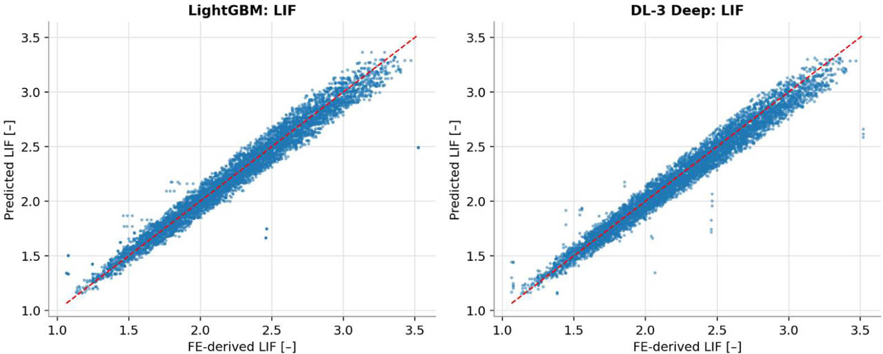
Figure 5:
Predicted versus FE-derived LIF for the selected LightGBM and DL-3 Deep models on the held-out test set
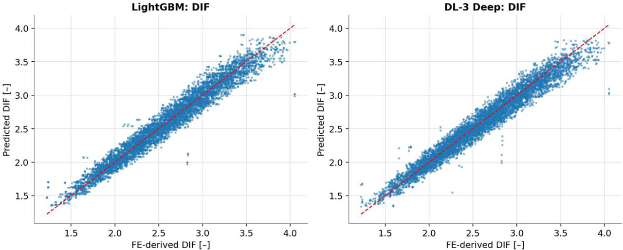
Figure 6:
Predicted versus FE-derived DIF for the selected LightGBM and DL-3 Deep models on the held-out test set
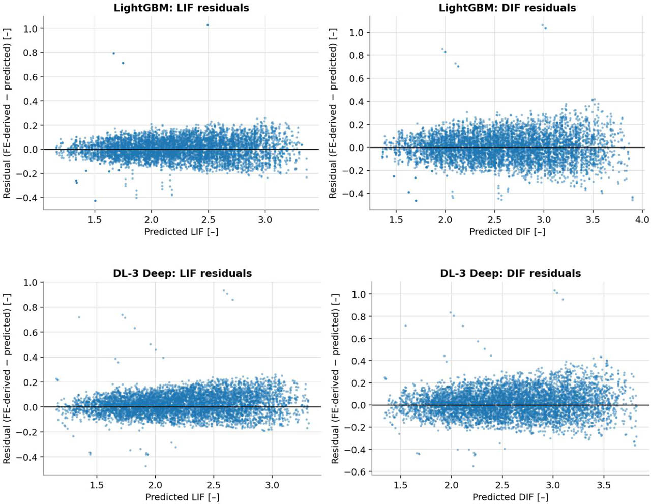
Figure 7:
Residual distributions for LIF and DIF predictions on the held-out test set, for LightGBM (top) and DL-3 Deep (bottom)
The predicted-versus-FE-derived scatter clusters tightly along the line of equality for both LIF and DIF in Figures 5 and 6, and the corresponding residuals in Figure 7 are centered on zero with no systematic trend visible across the prediction range, indicating that neither selected model exhibits meaningful bias toward over- or under-prediction at either the low or high end of the target range.
4.3. Generalization Behavior Across the Parametric Grid
The generalization pattern in Table 11 provides a useful diagnostic given the structured, factorial nature of the underlying dataset described in Section 3.2. Because the training grid is composed of configurations that frequently differ from their neighbours by a single parameter increment, for example, an adjacent number-of-stories value at otherwise identical geometry, models with high representational capacity and few constraints on complexity, notably the random forest, are able to memorise the fine-grained structure of the training grid rather than learning the smoother underlying relationship between geometry, loading, and collapse resistance. This is consistent with the random forest's very large train–validation gap in Table 11 (0.0391 for LIF and 0.0574 for DIF), which remains large even though all scenario records of a configuration are kept in the same partition.
By contrast, DL-3 Deep, with gaps of 0.0033 and 0.0029, and the other boosted and neural models with small gaps demonstrate that strong predictive accuracy on this parametrically structured dataset is achievable without relying on memorization of individual grid points. LightGBM and XGBoost lie at the boundary of the criterion on the single configuration-level split (LIF gaps of 0.0110 and 0.0132), but both show smaller gaps under grouped cross-validation (0.0056 and 0.0080 for LIF; Table 10). This supports the validity of the overfitting-aware selection criterion adopted in Section 3.6 as a meaningful safeguard specific to factorially generated datasets of this kind, where the risk of a model learning the sampling grid itself, rather than the physical relationship it was designed to approximate, is elevated relative to a purely randomly sampled dataset.
4.4. Illustrative Comparison on a Random Subsample
To provide an additional, visually interpretable check on model behaviour beyond the aggregate metrics in Table 11, predictions from all eleven benchmarked models were also examined on a random subsample of 22 configurations drawn from the held-out test set. This subsample is presented purely for illustration: because Table 11 already reports the full 6,578-record test-set metrics used for model selection and reporting throughout this study, the R2 and MAE values annotated in Figures 8–11 below are computed on this small illustrative subsample only, and are not directly comparable to, nor a replacement for, the full test-set values in Table 11.
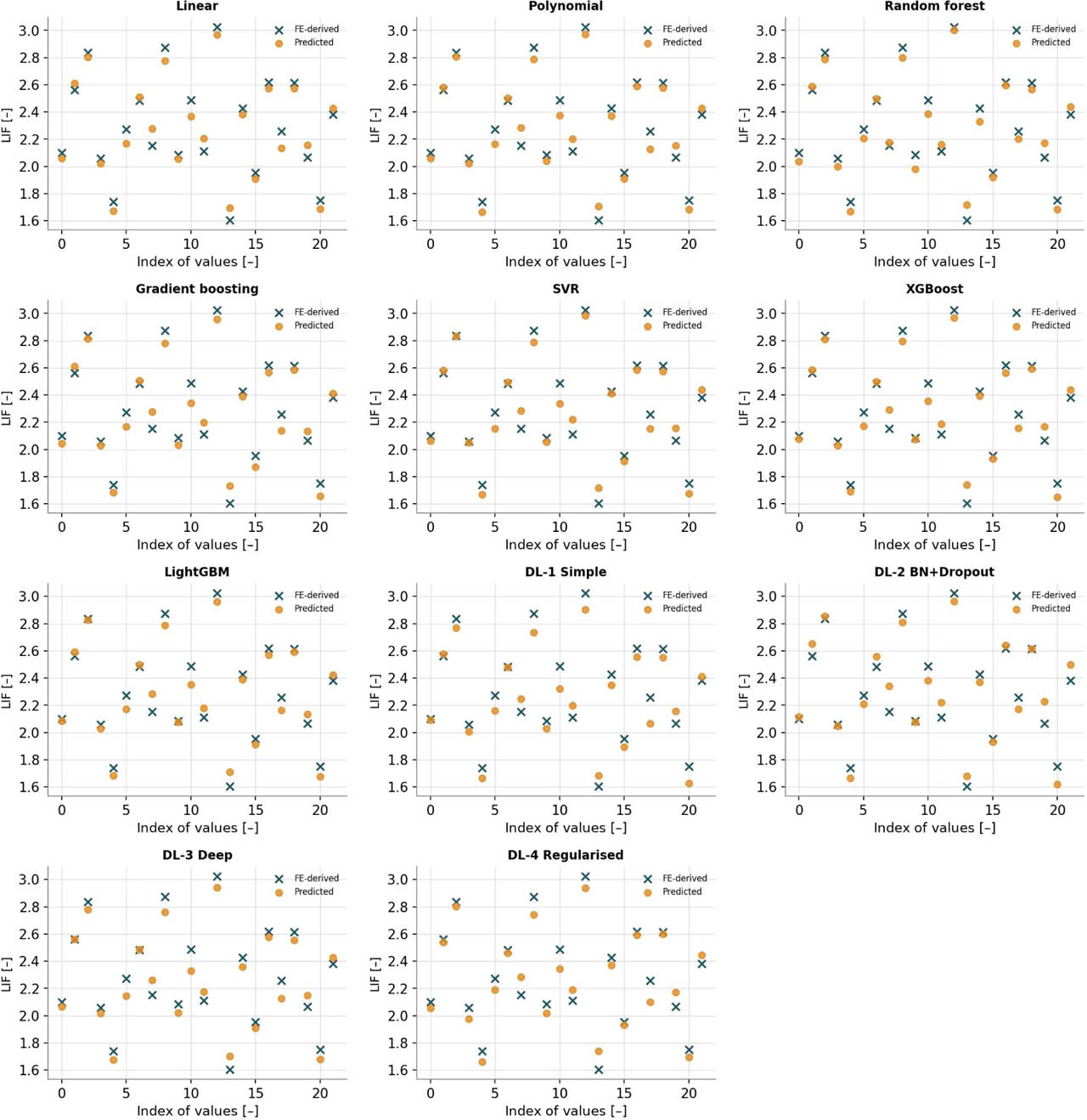
Figure 8:
Predicted versus FE-derived LIF for all eleven benchmarked models on a random subsample of 22 held-out test-set configurations
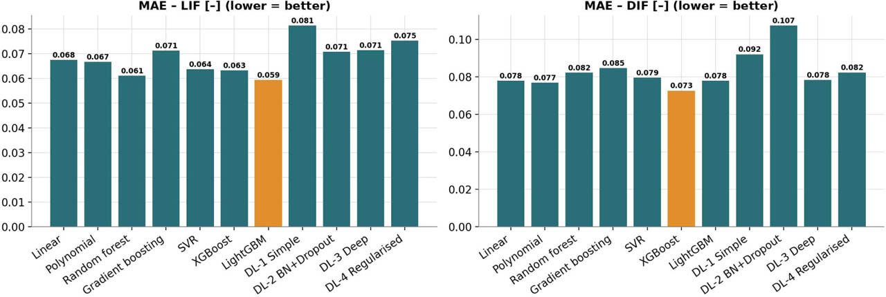
Figure 9:
Mean absolute error (MAE) for LIF and DIF across all eleven models, computed on the 22-configuration illustrative subsample
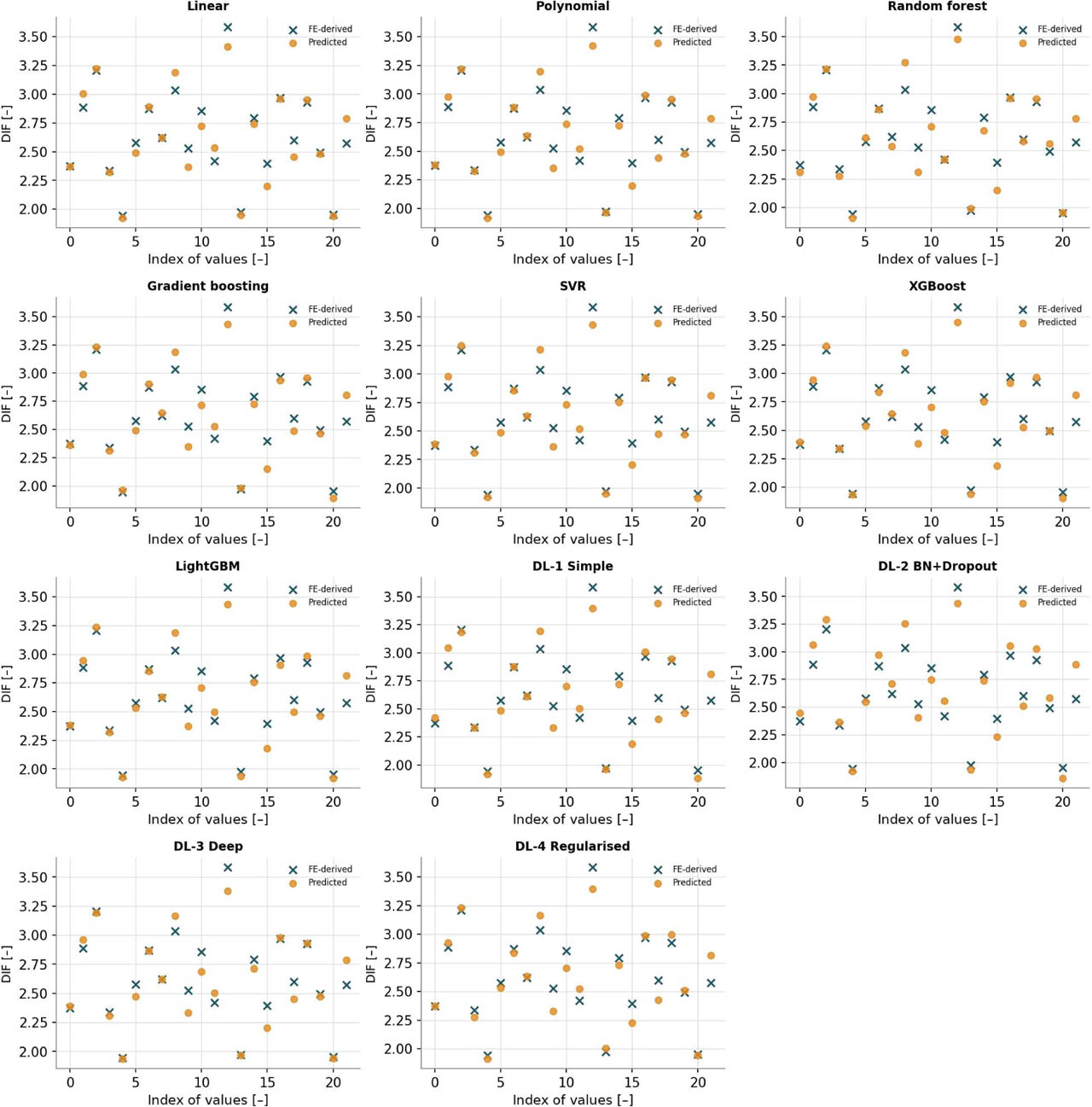
Figure 10:
Predicted versus FE-derived DIF for all eleven benchmarked models on a random subsample of 22 held-out test-set configurations
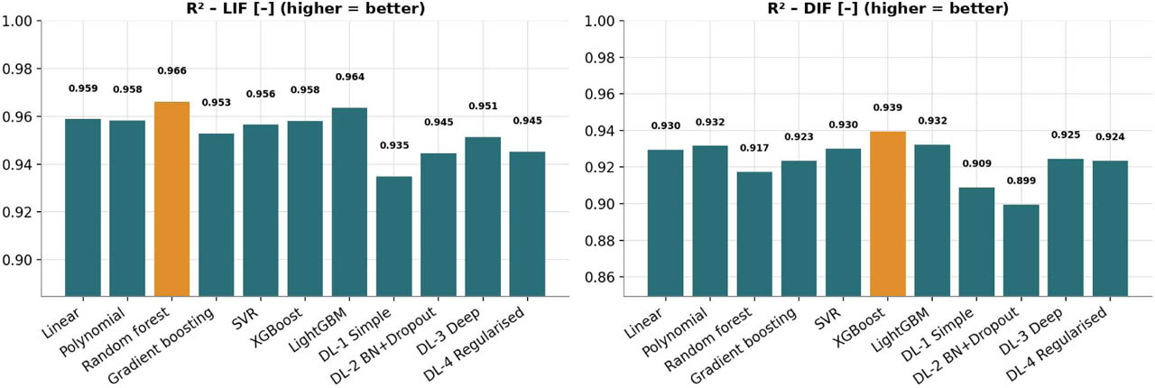
Figure 11:
Coefficient of determination (R2) for LIF and DIF across all eleven models, computed on the 22-configuration illustrative subsample
Consistent with the full test-set results in Table 11, the illustrative subsample confirms that all eleven models track the FE-derived LIF and DIF values closely at the level of individual configurations, with no model exhibiting systematic bias toward over- or under-prediction across the sampled range.
4.5. Sensitivity of Predictions to Input Parameters
Two complementary analyses were used to examine which input parameters most strongly govern the predicted collapse-resistance indicators. First, the statistical association between each input and each target was computed across the full dataset: the absolute Pearson correlation coefficient |r| for the numerical inputs, which measures linear association only, and the correlation ratio (η) for the categorical column removal location and load scenario. Figure 12 presents this association ranking. A correlation coefficient measures the strength of association, not the change in response per unit change in an input, and may miss non-linear or interacting effects; it is therefore not interpreted here as sensitivity. Second, the sensitivity of the trained LightGBM model was quantified on the test set with SHAP values and with permutation importance, defined as the drop in test R2 when one input is randomly shuffled. Table 12 reports both measures, and Figures 13 and 14 show the SHAP summary plots for LIF and DIF.
Table 12:
Model-based sensitivity of the LightGBM predictions on the test set: mean absolute SHAP value and permutation importance (drop in R2)
| Input | Mean |SHAP| LIF [–] | Mean |SHAP| DIF [–] | Permutation ΔR2 LIF [–] | Permutation ΔR2 DIF [–] |
|---|---|---|---|---|
| Number of stories | 0.373 | 0.429 | 1.607 | 1.600 |
| Bay span | 0.135 | 0.157 | 0.231 | 0.231 |
| Number of bays | 0.111 | 0.129 | 0.163 | 0.164 |
| Story height | 0.005 | 0.007 | 0.014 | 0.015 |
| Column removal location | 0.005 | 0.006 | 0.013 | 0.013 |
| Load scenario | 0.000 | 0.000 | 0.000 | 0.000 |
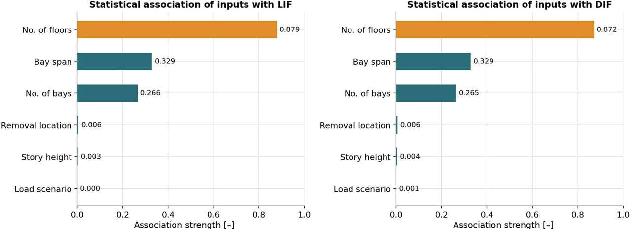
Figure 12:
Statistical association of inputs with LIF and DIF (|Pearson r| for numerical inputs; correlation ratio η for categorical inputs)
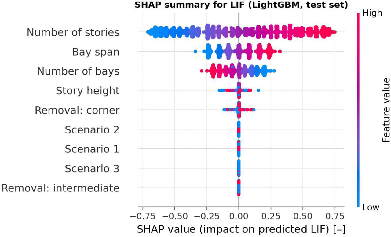
Figure 13:
SHAP summary plot for LIF (LightGBM, test set)
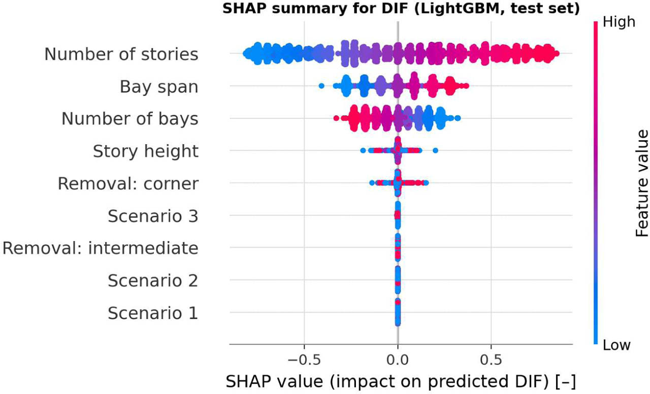
Figure 14:
SHAP summary plot for DIF (LightGBM, test set)
Number of stories emerges as the dominant driver of both LIF and DIF, consistent with the physical expectation that taller frames redistribute load through a greater number of alternate paths following column removal. Bay span and number of bays exert a secondary but non-negligible influence, while story height and column-removal location contribute comparatively little to the variance in either target. The association ranking is consistent with established structural-mechanics intuition and supports the physical plausibility of the relationships learned by the surrogate models.
The SHAP and permutation measures in Table 12 rank the inputs in the same order. The number of stories dominates (mean |SHAP| of 0.373 for LIF and 0.429 for DIF), followed by bay span (0.135 and 0.157) and number of bays (0.111 and 0.129); story height and column removal location contribute marginally. The load scenario has no measurable importance in the reported LightGBM sensitivity analysis, which is consistent with the dataset itself, in which the three scenarios change LIF and DIF by less than ±3%.
The direction of the bay-span relationship is further illustrated in Figure 15, which plots LIF and DIF respectively against bay span across the full dataset, disaggregated by column-removal location. Both indicators increase with bay span, reflecting the larger tributary areas and correspondingly higher demand on the frame following removal of a column at longer spans.
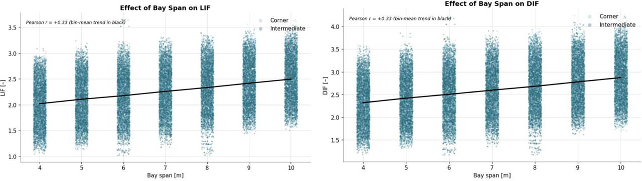
Figure 15:
Effect of bay span on LIF and DIF across the full dataset, by column-removal location
5. Discussion, Deployment, and Limitations
5.1. Practical Interpretation of the Selected Models
The practical significance of the results in Table 11 is best understood by analogy to a familiar engineering tool. LightGBM and the deep neural network, DL-3 Deep, together function as a pre-verified design chart, calibrated on 23,019 training records and validated on a further 9,867 held-out records, that replaces the need to run a full nonlinear FE analysis for every new building configuration falling within the trained parameter space. Where a design chart in a code annex encodes numerically derived results into a lookup table, the surrogate models developed here encode the same class of information into a trained function: an engineer supplies six geometric and loading parameters and receives predicted LIF and DIF values within a fraction of a second, at a typical error under 3% relative to the underlying FE benchmark, rather than constructing and solving a nonlinear FE model for every case.
DL-3 Deep is recommended as the primary surrogate on the basis of the highest test accuracy of all eleven candidates (R2 = 0.9714 for LIF, 0.9576 for DIF) combined with a train–validation gap well below 0.01 (0.0033 and 0.0029), and it is the architecture deployed in the decision-support platform described in Section 5.3. LightGBM is recommended as the classical alternative, achieving comparable accuracy (R2 = 0.9664 for LIF, 0.9535 for DIF) with straightforward deployment that does not require a deep learning framework, although its generalization gap on the single configuration-level split lies marginally above 0.01 for LIF.
As an illustration, consider a fifteen-story frame with a 4 m story height, a 6 m bay span, four bays, a corner column removal scenario, and load scenario 2. Supplying these six parameters to either selected model returns predicted LIF and DIF values in well under a second, values that would otherwise require constructing and solving a full nonlinear FE model to obtain. This is the practical value proposition of the framework: not a replacement for FE analysis in validation or research contexts, but a rapid screening and preliminary design tool calibrated against it.
5.2. Engineering Validation via a Case Study
To validate the selected models beyond aggregate test-set metrics, six configurations spanning the validated domain (2 to 28 stories, story heights of 3 to 5 m, bay spans of 5 to 10 m, 3 to 9 bays, corner and intermediate column removal, and all three load scenarios) were taken from the held-out test partition, so that none of them was used for training, and their FE-derived LIF and DIF were compared with the surrogate predictions. Table 13 presents this comparison. DL-3 Deep reproduced LIF and DIF with mean absolute deviations of 3.76% and 3.74% (maximum 6.9%), consistent with its test-set MAPE, while LightGBM showed mean absolute deviations of 5.70% for LIF and 3.45% for DIF.
Table 13:
Comparison of FE-derived LIF and DIF with DL-3 Deep and LightGBM predictions for six held-out configurations. Δ is the percentage deviation of the prediction from the FE-derived value; S1 to S3 denote load scenarios 1 to 3
| Configuration (stories / height / span / bays / location / scenario) | FE LIF [–] | FE DIF [–] | DL-3 LIF [–] | Δ [%] | DL-3 DIF [–] | Δ [%] | LightGBM LIF Δ [%] | LightGBM DIF Δ [%] |
|---|---|---|---|---|---|---|---|---|
| 3 / 5 m / 8 m / 6 / Corner / S3 | 1.694 | 1.894 | 1.712 | +1.1 | 1.972 | +4.1 | −0.8 | +1.9 |
| 2 / 3 m / 6 m / 7 / Intermediate / S2 | 1.524 | 1.775 | 1.492 | −2.1 | 1.715 | −3.4 | +16.2 | +6.9 |
| 10 / 4 m / 9 m / 5 / Intermediate / S1 | 2.065 | 2.425 | 2.184 | +5.7 | 2.523 | +4.0 | +4.3 | +1.9 |
| 16 / 3 m / 5 m / 5 / Intermediate / S3 | 2.318 | 2.488 | 2.158 | −6.9 | 2.496 | +0.3 | −6.5 | +0.2 |
| 28 / 3 m / 9 m / 9 / Intermediate / S1 | 3.019 | 3.413 | 2.843 | −5.8 | 3.278 | −4.0 | −4.7 | −2.5 |
| 28 / 3 m / 10 m / 3 / Corner / S1 | 3.237 | 3.966 | 3.209 | −0.9 | 3.702 | −6.7 | −1.8 | −7.3 |
| Mean absolute deviation | 3.76 | 3.74 | 5.70 | 3.45 |
The six comparisons show no systematic bias of either model with storey count, bay span or removal location. The largest deviations of DL-3 Deep are +5.7% for the 10-storey LIF, −6.9% for the 16-storey LIF and −6.7% for the DIF of the 28-storey, 10 m span corner case, whereas the largest LightGBM deviation is +16.2% for the LIF of the two-storey frame, at the lower boundary of the storey range. FE-derived values in Table 13 are taken from the nonlinear analyses of the dataset and were not used for training. Six configurations cannot substitute for validation across the full trained parameter space, and further independent nonlinear analyses spanning the range established in Section 3.2 remain valuable.
5.3. Deployment as a Web-Based Decision-Support Platform
The selected deep neural network, DL-3 Deep, is deployed as a publicly accessible, web-based decision-support platform at https://huggingface.co/spaces/Amromansour1985/AI_Structural_collapse, offering both single-configuration prediction and batch prediction from an uploaded file of multiple configurations, together with automated risk-band classification of the predicted LIF and DIF values into descriptive categories to support rapid engineering triage, as illustrated in Figures 16 and 17 respectively. The platform accepts only inputs within the validated domain; story heights other than 3, 4 or 5 m are rejected.

Figure 16:
Interface of the deployed web-based decision-support platform, showing the single-configuration prediction view, with input geometry, preprocessed feature vector, and classified LIF and DIF outputs
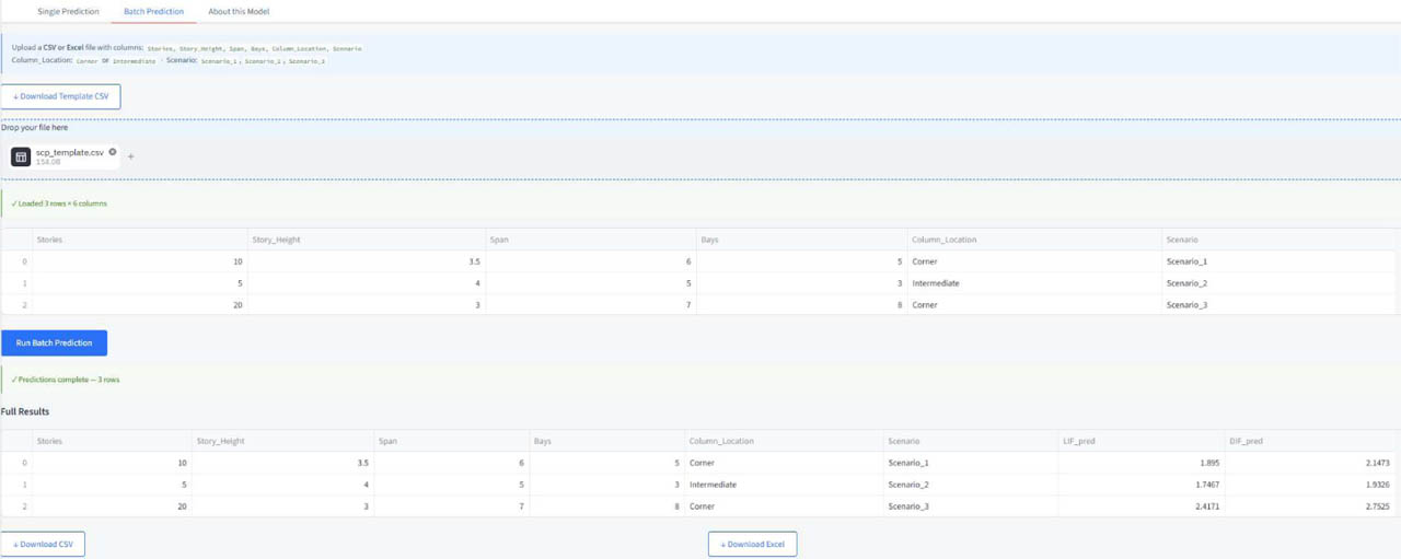
Figure 17:
Interface of the deployed web-based decision-support platform, showing the batch-prediction view with risk-band classification
5.4. Validity Range and Limitations
The following limitations must be stated clearly alongside the capability demonstrated in this study. First, and most importantly, the models are validated only within the parameter space represented in the training data, specifically 2 to 30 storeys, story heights of 3, 4, or 5 m, bay spans of 4 to 10 m, and 2 to 10 bays, as established in Section 3.2. Predictions for configurations outside this range constitute extrapolation rather than the interpolation the models were validated for. Consistent with this, it is recommended that the deployed platform described in Section 5.3 restrict its accepted input range to this validated envelope, rather than exposing a wider input range that would permit unvalidated extrapolation; any future extension of the platform's accepted input range should be accompanied by a corresponding extension of the training dataset and re-validation of model performance across the new range, rather than treated as a simple interface change.
Second, the underlying dataset is simulation based, and the reported accuracy in Section 4 and the comparison in Section 5.2 reflect agreement with the FE benchmark rather than independent validation against physical test measurements; use in design practice should be accompanied by appropriate engineering review. Third, the case-level comparison in Section 5.2 rests on six held-out configurations drawn from the same parametric dataset; extending this validation to independently generated nonlinear analyses spanning multiple points across the trained parameter space, particularly toward its boundaries, where the two-storey case shows reduced LightGBM accuracy, remains a priority for future work, together with extending the framework beyond the structural typology considered here and validating the deployed platform's risk-band classification thresholds against engineering judgement on a set of independently reviewed case studies.
Finally, the load scenario has no measurable influence on the predictions (Section 4.5), because the three scenarios change LIF and DIF by less than ±3% in the dataset; the models cannot therefore be used to discriminate between load patterns. In addition, the nonlinear-analysis settings listed as reconstructed in Section 3.2.1 define a reference modelling basis rather than recovered values, which limits strict reproduction of the dataset labels.
6. Conclusion and Future Work
6.1. Summary of Findings
This study set out to address a persistent gap between the regulatory requirement for explicit progressive collapse assessment and the practical difficulty of meeting that requirement through conventional nonlinear finite element (FE) analysis alone. A structured parametric study, varying five geometric and configurational parameters, number of stories, story height, bay span, number of bays, and column removal location, across three load scenarios, produced 10,962 base building configurations and 32,886 configuration–scenario combinations. The resulting database contains 32,886 configuration–scenario records, each jointly labelled with the Load Increase Factor (LIF) and the Dynamic Increase Factor (DIF).
Eleven candidate surrogate models, seven classical machine learning algorithms and four deep neural network architectures, were benchmarked under identical preprocessing and a configuration-level partitioning in which all load scenarios of a configuration remain in the same partition. Selection was governed not by raw test accuracy alone but by an explicit overfitting-aware criterion requiring the gap between training and validation performance to remain below 0.01. This criterion proved decisive: the random forest fitted the training data almost perfectly but showed a train–validation gap four to five times larger than any other model, a result interpreted in Section 4.3 as evidence of memorization of the parametric grid rather than genuine generalization. DL-3 Deep achieved the highest test-set accuracy with a gap well below 0.01 (R2 = 0.9714 for LIF and 0.9576 for DIF), and LightGBM was the best classical benchmark (R2 = 0.9664 and 0.9535).
Both selected models were subsequently compared with FE-derived values for six held-out configurations spanning the validated domain, DL-3 Deep reproducing LIF and DIF with mean absolute deviations of 3.76% and 3.74% (maximum 6.9%), consistent with the aggregate accuracy reported on the held-out test set. DL-3 Deep was deployed as a publicly accessible, web-based decision-support platform, offering single-configuration and batch prediction with automated risk-band classification and returning a prediction in about 0.05 s per configuration.
6.2. Contributions
Set against the threefold novelty claimed at the outset of this study, each contribution has been delivered and demonstrated across the preceding sections. First, the large-scale parametric database developed in Section 3, approximately eight times larger than comparable datasets identified in the literature reviewed in Section 2, provides a systematically structured foundation for surrogate model training that avoids the ad hoc or opportunistically sampled datasets characteristic of much prior work in this area. Second, the overfitting-aware model selection procedure adopted throughout Sections 3 and 4 provides a concrete, reproducible safeguard against the specific risk, identified in Section 4.3, that a high-capacity model trained on a factorially structured dataset may achieve deceptively high accuracy through memorization of the sampling grid rather than the underlying physical relationship. Third, the identification, validation, and deployment of two accurate, generalizing surrogate models, LightGBM and DL-3 Deep, closes the gap between numerical feasibility and practical engineering use that was identified in Section 2 as a shortfall in the existing body of machine learning research on progressive collapse.
Taken together, these contributions position the present study as an advance beyond the authors' own precursor feasibility investigation (Mansour et al., 2025), extending a single-indicator, moderate-scale demonstration into a dual-indicator, rigorously validated, and operationally deployed framework.
6.3. Limitations and Future Work
The limitations discussed in full in Section 5.4 define the boundaries of the present study's applicability and the corresponding priorities for future research. The models developed here are validated only within the parameter space represented in the training data, specifically 2 to 30 storeys, story heights of 3, 4, or 5 m, bay spans of 4 to 10 m, and 2 to 10 bays; extending the validated range to taller buildings, wider spans, unequal bay spans or a continuous rather than discrete treatment of story height would require a corresponding extension of the underlying parametric dataset and re-validation, not merely an adjustment to the deployed interface. The underlying dataset is simulation based throughout, and no comparison against physical experimental data has yet been undertaken; incorporating physical test benchmarks, where available, would strengthen confidence in the framework's applicability beyond numerical agreement. The case-level comparison reported in this study rests on six held-out configurations drawn from the same dataset; extending it to independent nonlinear analyses across the trained parameter space, particularly toward its boundaries, remains an immediate priority. Finally, fire-induced thermal loading is not covered by the present models.
Beyond these three specific limitations, the framework's scope in its current form is restricted to steel moment frames under column removal scenarios. Extending the underlying methodology, structured parametric data generation coupled with overfitting-aware surrogate model selection, to other structural typologies and lateral load-resisting systems represents a natural direction for future work, as does extending the SHAP-based interpretability analysis of Section 4.5, currently applied to LightGBM, to the deployed deep learning model.
6.4. Concluding Remarks
This study has demonstrated that a rigorously generated parametric dataset, combined with a model selection procedure that explicitly guards against overfitting, can produce surrogate models capable of predicting progressive collapse resistance indicators for multi-storey steel moment frames with accuracy approaching that of direct nonlinear FE analysis, at a small fraction of the computational cost. By carrying the resulting model through to a publicly deployed, interactive platform, this work moves beyond a purely academic demonstration of feasibility toward a tool with direct utility in routine structural design practice. As the volume and structure of simulation-generated engineering data continues to grow, the approach demonstrated here, systematic dataset generation, disciplined model selection, and case-level engineering validation prior to deployment, offers a template applicable well beyond the specific problem of progressive collapse, contributing toward the broader digitalization of structural safety evaluation within the AEC industry.
Acknowledgements
This research received no specific grant from any funding agency in the public, commercial, or not-for-profit sectors.
Notes
[1] Contributed by Author Contributions
A.M. conceived and designed the study, developed the parametric dataset generation framework, conducted the machine learning and deep learning model benchmarking, and drafted the manuscript. M.H.S. contributed to the structural engineering methodology and supervised the finite element analysis campaign. A.B. contributed to the machine learning and deep learning model architecture and evaluation methodology. S.A.M. contributed to data interpretation, engineering validation of the case study, and manuscript review. All authors critically reviewed and approved the final version of the manuscript and agreed to be accountable for all aspects of the work.