

1. Introduction
As a widely used discontinuous numerical analysis method, Particle flow code (PFC) uses finite-size particles to express materials, and the mechanical behavior of the materials are simulated by the interaction between particles. In the field of the geotechnical engineering, it is widely used to simulate the mechanical behavior tunnel, bridge, or slope (Xiang et al. 2018; Li et al. 2022a; Huang et al. 2015, Cen et al. 2017; Li et al. 2022b; Su et al. 2026), because of its advantages of easily handling large deformation size and discontinuous materials (Wu et al. 2020; Francis et al. 2023).
In geotechnical engineering, the properties of rock and soil materials are expressed by parameters, such as the uniaxial compressive strength, tensile strength, cohesion intercept, and friction angle, which are always obtain by laboratory test. One of the main tasks of the numerical simulation is to establish numerical models with known rock or soil parameters. However, in PFC, the material parameters cannot be defined directly, they are determined by micro-parameters, such as cohesion, effective modules, which are used to describe the interaction between particles. Therefore, suitable micro-parameters should be selected before establishing the numerical model, which is called parameter calibration.
In order to accurately calibrate the micro-parameter of the numerical models, there are numbers of methods are proposed, such as trail-and-error (Xia and Zeng 2018; Castro-Filgueira et al. 2017; Tong et al. 2019; Potyondy et al. 2004; Ibarra et al. 2022), regression (Xu et al. 2022; Yoon 2007; Chehreghani et al. 2017; Deng et al. 2019; Pan et al. 2021; Hu et al. 2023; Wang 2020a; He 2018; Wang et al. 2020b; Dong and Li 2022; Chi et al. 2022; Li et al. 2023; Hao et al. 2022; Dong 2022), and artificial intelligence (Ma 2020; Shentu and Lin 2023; Qu et al. 2019, 2020; Cheng et al. 2019; Simone et al. 2019; Wu and Huang 2023; Zhong et al. 2023; Li et al. 2021; Ji et al. 2022). The mentioned methods obtained acceptable results, which is significant to establish accurate numerical model.
Generally, in terms of a rock model with known strength parameters, there are multiple combinations of micro-parameter matched. In other words, the selection of micro-parameters has non-uniqueness (Ni et al. 2025a, 2025b). Current method can be used to select a micro-parameter combination matched known strength parameter instead of the only combination. In this respect, the non-uniqueness of the micro-parameter solutions needs to be suppressed.
Applying constraints is one of the effective measures to suppress the non-uniqueness of solutions (Wang 2020). In fact, during simulating the rock test, the distribution of the generated fractures also shows significant difference and be affected by the micro-parameters. Therefore, classifying the generated fracture morphology, and establishing the relationship between the fracture morphology and the micro-parameters, and involving the relationship into the parameter calibration as constraints, is helpful for suppressing the non-uniqueness of the micro-parameters and establishing accurate numerical rock model, and it is also the main contribution and innovation of this research.
The main task of this research is to study the fracture morphology generated in the simulation of rock mechanical test, including the uniaxial compression test, the Brazilian splitting test, and the direct shear test based on multiple numerical models with different micro-parameters. On this basis, the generated fractures are divided into several groups, and the relationship between the morphology and the micro-parameters are researched. In addition, a method for evaluating fracture morphology based on K-nearest neighbors is proposed and verified, which can evaluate the fracture morphology generated in simulating the rock test, and the time cost of the simulation can be saved. This research might be helpful for providing reasonable constraints to suppress the non-uniqueness of the micro-parameters and establishing accurate numerical rock models.
2. Rock mechanical test in PFC
This research mainly studies the fracture morphology of the rock numerical models generated by uniaxial compression test, Brazilian splitting test, and direct shear test. For this target, totally 1517 rock numerical models are established with different micro-parameter combinations and used to conduct the above rock mechanical tests. Thus, the fracture morphologies and different micro-parameters are obtained, which is the data foundation of this research.
In the established rock numerical model, the linear parallel bonding model is used to characterize the mechanical behavior between particles, as shown in Figure 1. The balls are connected by a linear contact bond, a parallel contact bond and a damping element in the bonded state. The parallel contact bond has specified tensile and shear strengths. In a numerical rock model composed of particles and bonds, the porosity determines their numbers, and also determines the strength parameter and the fracture morphology. In addition, the bond can withstand normal tensile force and tangential shear force, whose magnitude is determined by the effective modulus, friction angle, tensile strength and cohesion force of bonds. The force and failure of the numerical model follows the Mohr-Coulomb criterion, the shear force between particles linearly increase with the normal force increasing, and the coefficient, also the friction angle, is also influencing the strength between particles. In addition, the radius multiplier, the ratio between normal and tangential stiffness, also affects the failure of bonds.
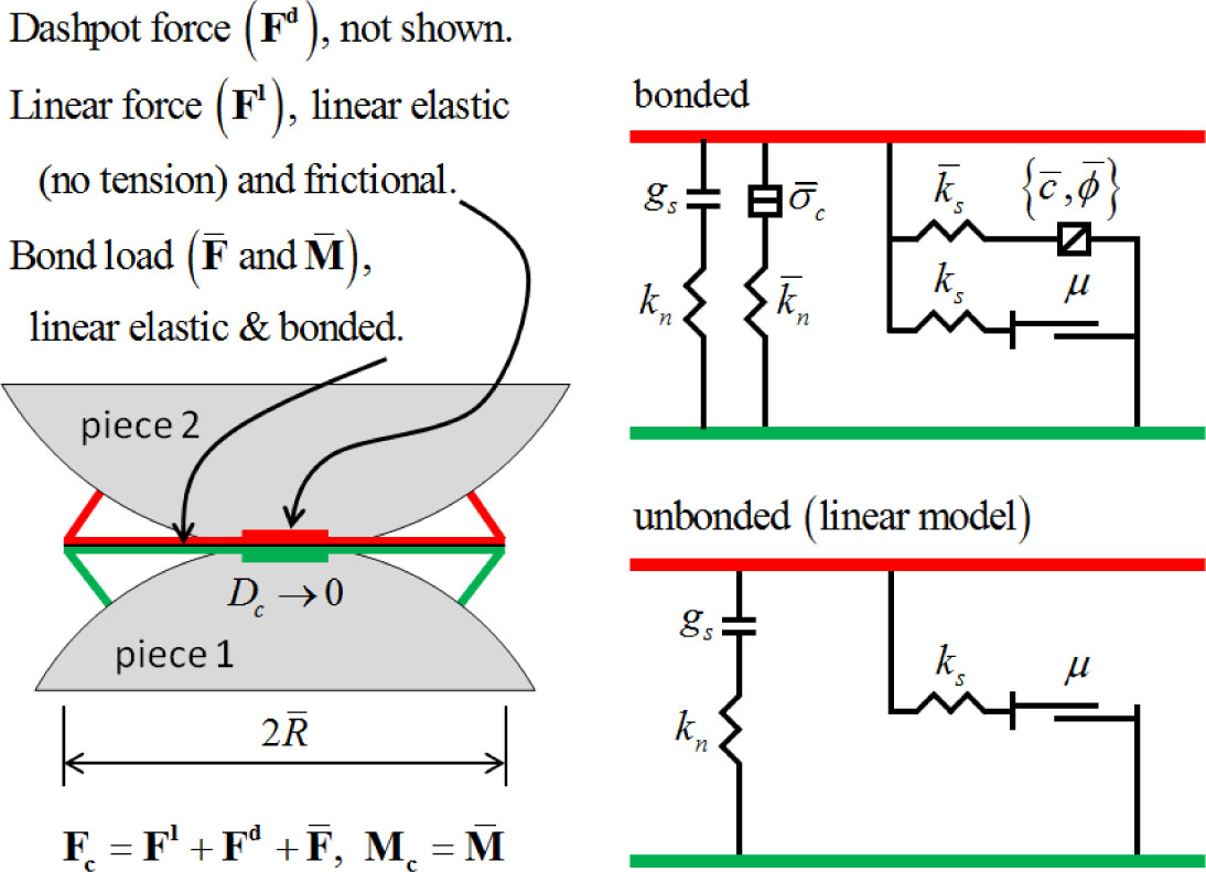
Figure 1:
Schematic diagram of the 2D linear parallel bonding model (Ni et al. 2025a, 2025b)
According to above analysis and previous researches, the main micro-parameters that have significant influences on the contact between particles are tensile strength between particles (σmi), cohesion force between particles (cmi), radius multiplier (λmi), effective modulus ( ), friction angle (ϕmi), friction coefficient(μmi), and porosity (pmi). Those micro-parameters are also used as the independent variable to established totally 1517 rock numerical models, and their ranges are listed in Table 1.
Table 1:
Ranges of each input micro-parameters (Ni et al. 2025a, 2025b)
| Input | Symbol | Unit | Lower bounds | Upper bounds |
|---|---|---|---|---|
| Tensile strength | σmi | [MPa] | 10 | 90 |
| Cohesion force | cmi | [MPa] | 10 | 90 |
| Radius multiplier | λmi | - | 0.5 | 1 |
| Effective modulus | [GPa] | 10 | 90 | |
| Friction angle | ϕmi | [°] | 40 | 60 |
| Friction coefficient | μmi | - | 0.1 | 0.9 |
| Porosity | pmi | - | 0.1 | 0.15 |
In the range listed in Table 1, 1517 micro-parameter combinations are randomly selected and generate rock numerical models, and these models are used to conduct the uniaxial compression test, Brazilian splitting test, and direct shear test, which is shown in Figure 2.
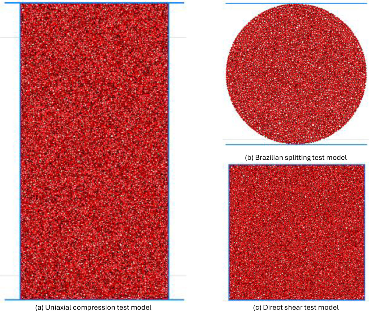
Figure 2:
Numerical models for data collection (Ni et al. 2025a, 2025b)
As shown in Figure 2(a), the numerical rock model used in the uniaxial compression test is shown as a rectangle, with the height of 100mm and width of 50mm.and the loading speed of 0.01m/s. As shown in Figure 2(b) and (c), the numerical model used in the Brazilian splitting test is shown as a circle with the diameter of 50mm, and the one used in the direct shear test is a square with the side length of 50mm. The loading speed in both the Brazilian splitting test and the direct shear test is 0.01m/s. During the simulation, the normal or tangential loading of each iteration is recorded. When the loading decreases to lower than the historical highest load, the simulation is end, and the corresponding fracture morphologies is recorded.
After each test simulation, the fracture morphology corresponding to each micro-parameter combination is qualitatively determined according to macroscopic distribution features of the generated cracks. These simulation results are used to analyze the relationship between the fracture morphologies and the micro-parameters.
3. Classification of the fracture morphology
The aiming of this paper is to research the relationship between the micro-parameters of rock numerical model and the fracture morphologies generated by rock mechanic tests, such as the uniaxial compression test, Brazilian splitting test, and the direct shear test. To completely describe the possible fracture morphologies generated by rock test, totally 1517 series of rock numerical models are established and involved to the simulation process shown in Figure 2. All of the fractures morphology results are summarized as several kinds, and each one is introduced in this section.
3.1. Fracture morphology in uniaxial compression test
According to the simulation results of the uniaxial compression test, all of the 1517 series of results are divided into three groups. The schematic figures and simulation results are shown in Figure 3
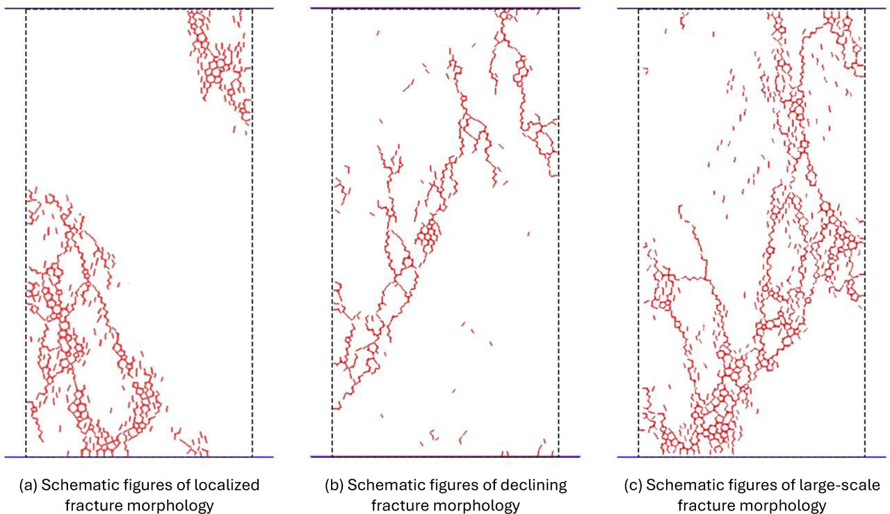
Figure 3:
Schematic figures of different fracture morphology generated in the uniaxial compression test
Localized fracture morphology
As Figure 3 (a) shows, one of the most significant characters of the localized fracture morphology is that there is no penetrating damage occurred inside the numerical samples. Under this morphology type, most fractures are concentrated at the upper and lower ends of the samples, especially near the four corners of the rectangle. When the localized fracture morphology occurs, the rock numerical model has not been completely destroyed. However, due to the localized damaged, the compressed area is reduced, and the stress is rapidly increased, and a large-scale damage of rock sample always occurred soon. Therefore, it can be approximately considered as completely failure of the rock when localized fracture morphology occurs.
Declining fracture morphology
In actual uniaxial compression test, samples with high strength and integrity always generate the fractures similar with Figure 3 (b). In declining fracture morphology, the fractures are concentrated on a slender strip, which penetrates the whole numerical model and always extends along a direction near 45°.
Large-scale fracture morphology
The rock numerical samples shown in Figure 3 (c) are completely destroyed, while the generated fractures occupied nearly the whole rectangle area. Generally, the large-scale fracture morphology always occurred in rock sample with relatively low strength parameters, especially the tensile strength and cohesive strength between particles.
3.2. Fracture morphology in Brazilian splitting test
Similar with the uniaxial compression test, the results of the Brazilian splitting test are also shown in three kinds of fracture morphologies, as shown in Figure 4.
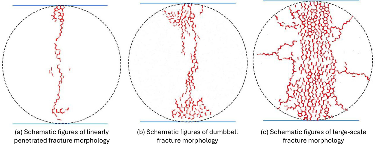
Figure 4:
Schematic figures of different fracture morphology generated in the Brazilian splitting test
Linearly penetrated fracture morphology
As shown in Figure 4 (a), linear penetrated fracture morphology is extended along the loading direction and penetrated through the circular cross-section, and most of the remaining area have no generated fractures. The fractures are mainly addressed in a slender area. It is the most common fractures pattern and consistent with the actual test of rock samples with high integrity.
Dumbbell fracture morphology
In the middle section, the generated fractures are distributed in a slender area and similar with the linearly penetrated fracture morphology. Differently, the generated fractures are distributed in large areas in the area near the contact point, also the top and bottom side of the sample. These areas are similar with sectors, and the whole fractures zone is similar with a dumbbell (Figure 4 (b)).
Large-scale fracture morphology
In terms of the large-scale fracture morphology (Figure 4 (c)), there are a large number of generated fractures, and their extend directions are always irregular, which results a large area of fractures distribution. In FPC2D, this kind of fracture morphology is always generated with high loading speed or low strength parameters.
3.3. Fracture morphology in direct shear test
According to the simulation results, the appeared fracture morphologies can be divided into two groups, as show in Figure 5.
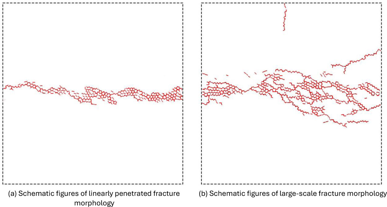
Figure 5:
Schematic figures of different fracture morphology generated in the direct shear test
Linearly penetrated fracture morphology
In terms of the rock with high strength and integrity, fractures extend along the horizontal axis of the sample are always occurred. Generally, the fracture zone of this kind is always narrow, as shown in Figure 5(a).
Large-scale fracture morphology
Differently, the direct shear test of rock with weak strength and integrity, always generate large-scale fracture morphology (Figure 5(b)), whose fracture zone is relatively wide. Although the extending direction of the fractures of the two morphologies are similar, the main differences between the two morphology is the width of the fracture zone.
3.4. Constraints of the fracture morphologies
To investigate the influence of the parameters of the numerical model on the fractures morphologies, the simulation results should be classified according to their fracture morphologies. Before it, criteria of different morphologies are proposed according to the main fracture distribution.
To quantitatively identify the different fracture morphology, the distribution area of the 80% simulated fractures is used as the quantitatively criterion. In detail, as Figure 6 shows, each fracture corresponds to a break of connect between a pair of particles. Accordingly, in PFC 2D, the number of fractures can be counted automatically.
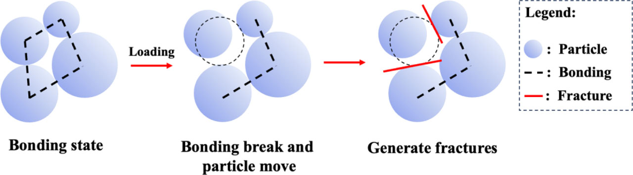
Figure 6:
Generation of fractures in PFC2D
Further, a proportion k is defined as the threshold of the proposed criteria. If the proportion of fracture located in specific area in the total fractures number are higher than k, the model will be judged as the corresponding classification. The criteria area corresponding to each fracture morphology classification is shown as Figure 7.
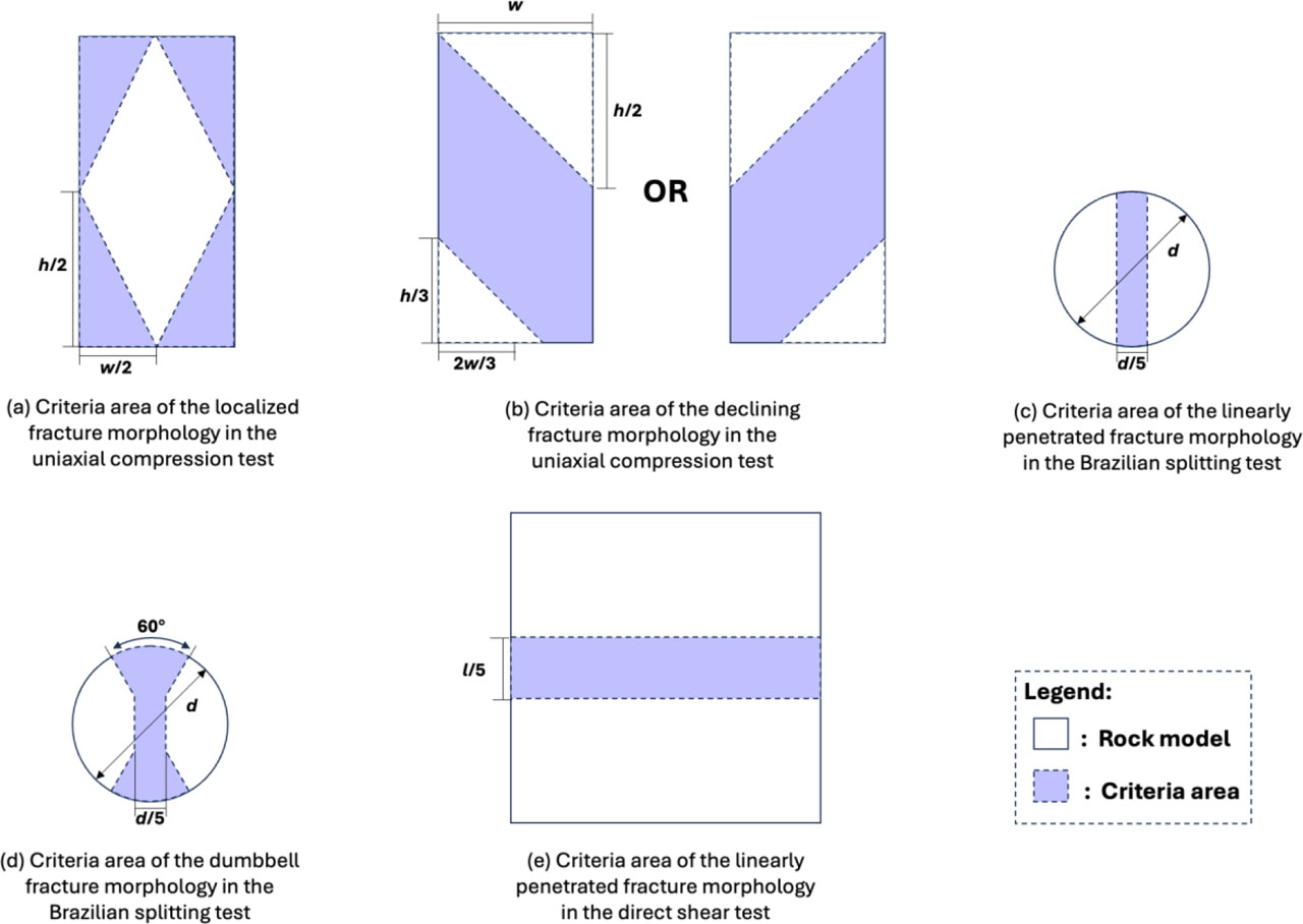
Figure 7:
The criteria areas of different fracture morphology
In Figure 7, w and h represent the width and height of the rock numerical model used in the uniaxial compression test, and d represent the diameter of the model used in the Brazilian splitting test, and l represent the length of the model used in the direct shear test. After simulation of the testing, if more than k of the total fractures is located in a criteria area, the model is judged as the corresponding fracture morphology. Take the localized fracture morphology as an example, assuming more than k fractures are located in the criteria area as Figure 7 (a) shows, also the four corners of the numerical model, the model is judged to generate localized fractures morphology after the uniaxial compression test. Specially, due to the large-scale fracture morphologies generated after the uniaxial compression test, the Brazilian splitting test, and the direct shear test are complex, and the generated fractures might be theoretically located in anywhere inside the numerical model, theoretically, there are no criteria area of the three kinds of morphologies. As alternatives, if there is more than (1-k) of the total generated fractures exceeding the criteria area shown in Figure 7, the model will be judged as the large-scale fracture morphology. For example, if less than k of the total fractures of a model generated by the uniaxial compression test are located in the area in both Figure 7(a) and (b), it is judged as the large-scale fracture morphology in uniaxial compressive test. Similarly, if less than k of the fractures generated in the Brazilian splitting test are located in Figure (c) and (d), it is also be judged as the large-scale fracture morphology. In addition, there are three kind of fracture morphologies of each rock numerical model established with the same micro-parameter combination, which is generated by the three tests, respectively, and the three morphologies are always independent.
4. Influence of micro-parameters on the fracture morphology
4.1. Distribution rules of the micro-parameters
Using the micro-parameter combinations listed in Table 1, totally 1517 rock numerical samples are established, and the corresponding tests are simulated. Take one of the numerical models as an example, with the micro-parameters are listed in Table 2, the simulated results are shown as Figure 8.
Table 2
Micro-parameter of the example numerical rock model
| σmi [MPa] | cmi [MPa] | λmi | ϕmi[°] | μmi | pmi | |
|---|---|---|---|---|---|---|
| 49.62 | 58.10 | 0.86 | 65.3 | 48.50 | 0.48 | 0.13 |
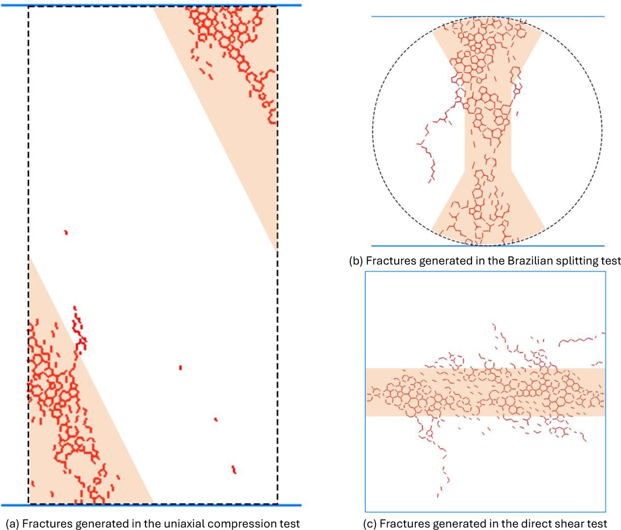
Figure 8:
Classification of the generated fractures morphology of the example model
To determine the fracture morphology of each numerical model clearly, the criteria k should be selected as a definite value. In this research, it is selected as 0.8. As Figure 8(a) shows, in the uniaxial compression test, there are totally 689 features generated. Among them, 632 features are located in the area shown in Figure 8(a), which accounts about 0.92. Therefore, the fracture morphology of the model generated in uniaxial compression test is recorded as the localized one. Similarly, there are totally 245 and 589 fractures generated in the Brazilian splitting test and the direct shear test, and 207 and 494 fractures are located in the area shown in Figure 8 (b) and (c), and accounts 0.85 and 0.84. Accordingly, it is judged as dumbbell and linearly penetrated fracture morphology. By analyzing the number and position of the generated fractures, the fracture morphologies are recorded. The number and the proportion of each morphology is listed in Table 3.
Table 3:
The proportion of each morphology
| Uniaxial compression test | Brazilian splitting test | Direct shear test | ||||||
|---|---|---|---|---|---|---|---|---|
| Morphology | Number | Proportion [%] | Morphology | Number | Proportion [%] | Morphology | Number | Proportion [%] |
| Localized | 163 | 10.7 | Linearly penetrated | 1122 | 74.0 | Linearly penetrated | 1287 | 84.8 |
| Declining | 914 | 60.3 | Dumbbell | 346 | 22.8 | Large-scale | 230 | 15.2 |
| Large-scale | 440 | 29.0 | Large-scale | 49 | 3.2 | |||
According to the statistic results, the declining morphology and the linear-penetrated morphology is the most frequently appeared morphology in uniaxial compression test, Brazilian splitting test, and the direct shear test, and the proportion of them is about 60.3%, 74.0%, and 84.8%, respectively. It is also consistent with regular test results. On this basis, the distribution rule of the micro-parameters of each morphology is further analyzed.
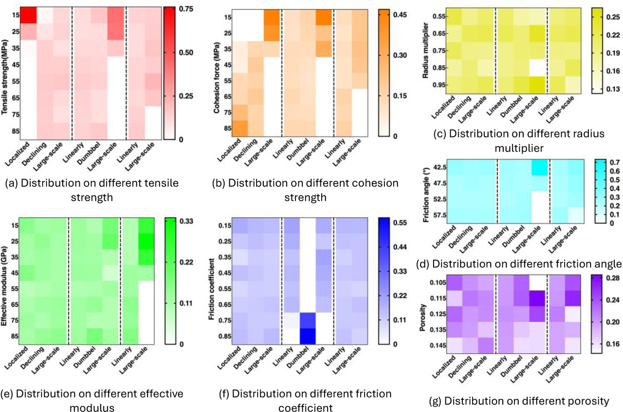
Figure 9:
Fracture morphology distribution on different micro-parameters
In Figure 9, the longitudinal coordinates represent the micro-parameters used by the numerical model, the horizontal coordinates represent the corresponding fracture morphologies. The color of the cubes represents the proportion of the samples number with corresponding ranges micro-parameters to the number of samples with the same morphology. In other words, the sum of the value corresponding to cubes in one column equals 1. As shown in Figure 9, it is found that the distribution of most fracture morphologies in the micro-parameter ranges are different. Take the tensile strength as an example (Figure 9 (a)), the darkest red cube shows that the tensile strength between particles of the most of localized fracture morphologies models are [10, 20] MPa, and the corresponding proportion is higher than 70%. Meanwhile, there is no localized fracture morphology generated with tensile strength between particles higher than 30 MPa. Similarly, the large-scale fracture morphology generated in the Brazilian splitting test is mainly occurred with low tensile strength between particles, mainly in the range of [10, 30] MPa. Compared with above two kinds of morphology, the distribution of the other morphologies in different tensile strength is relatively uniform, such as the linearly penetrated morphology generated in the Brazilian splitting test, as the corresponding frequency is close. It indicates that, in terms of the linearly morphology generated in the Brazilian splitting test, tensile strength between particles is not the primary influencing factor. According to the statistic results shown in Figure 9, the mainly influencing factors on each fracture morphology are listed in Table 4.
Table 4:
Primary influencing factors on each fracture morphology
| Rock test | Fracture morphology | Influencing factors |
|---|---|---|
| Uniaxial compression test | Localized | σmi, cmi |
| Declining | σmi, cmi | |
| Large-scale | cmi | |
| Brazilian splitting test | Linearly | μmi |
| Dumbbell | μmi | |
| Large-scale | σmi, cmi, ϕmi, μmi, pmi | |
| Direct shear test | Linearly | σmi, cmi |
| Large scale | σmi, cmi, , pmi |
4.2. Evaluating method of fracture morphology based on K-Nearest Neighbors
Based on the above analysis, there are significant impact of the micro-parameters of the numerical model on the fracture morphology. Accordingly, the fracture morphology of numerical models can be evaluated by their parameters before conducting simulations. During establishing numerical model, the micro-parameters always have multiple solutions, and the different micro-parameters always lead to different simulation results, such as the fracture morphology and failure loading. Therefore, evaluation of the fracture morphology is helpful for improving the accuracy of the numerical model.
Due to the large number of numerical samples and high sample density, a simple classification method should be selected to save calculation time consumption. Therefore, K-Nearest Neighbors is used to evaluate the fracture morphology with their micro-parameters as input. In detail, the seven micro-parameters are nondimensionalized to the range from 0 to 1 by 0–1 normalization (Wang et al. 2023; Meng et al. 2025). On this basis, Euclidean distance is used to evaluate the similarity of two samples, as shown in Eq.1.
Where:i and j - the order number of two samples,
Dij - the distance between ith and jth sample,
k – the order number
n - the total number of the model micro-parameter.
In this paper, n is selected as 7. In addition, yik and yjk is the kth micro-parameters of the ith and jth samples. The more the Dij, the larger distance between ith and jth sample, the more difference between the two samples. According to the Eq.1, the distance between a new unknown sample and any known sample can be calculated. To evaluate the fracture morphology of a new unknown numerical model, the Euclidean distances between it and all the 1517 known samples can be calculated, and the most frequent fracture morphology appeared in the nearest k samples are taken as the evaluated results of the unknown sample. Especially, if there are multiple kind of fracture morphology with equal occurrence times, the selected sample number k will be increased by 1. In this research, the number k is set as 10.
According to Eq.1, the nearest 10 samples can be distinguished. However, the simulated dataset applied on K-Nearest Neighbors is imbalanced, which may have negative influence on the evaluating results. Therefore, the number of nearest samples is modified by Eq.2 to balance the differences between the number of samples with different fracture morphology.
Where:and ni - the number of nearest samples with the ith fracture morphology,
wi - the weight of samples with the ith fracture morphology,
N and Ni – the total number of the dataset and sample with the ith fracture morphology,
C - the number of the fracture morphologies.
Especially, Eq.2 is independently calculated for each kind of rock test. Take the uniaxial compression test as an example, the N and the C is set as 1517 and 3, and the Ni of Localized, Declining, and Large-scale is set as 163, 914, and 440, respectively. Assuming that there is 2 Localized, 6 Declining, and 2 Large-scale samples is the nearest 10 samples, the weighted sample number of the three kind of sample is about 6.2, 3.3, and 2.3. Therefore, the fracture morphology of the assuming sample is evaluated as Localized instead of Declining. The weighted way can effectively avoid the shortcoming of samples being incorrectly evaluated as the majority fracture morphology due to dataset imbalance.
Table 5:
Micro-parameters of the example numerical model
| Model name | σmi [MPa] | cmi [MPa] | λmi | ϕmi [°] | μmi | pmi | |
|---|---|---|---|---|---|---|---|
| Example | 82.73 | 88.38 | 0.95 | 16.83 | 50.91 | 0.88 | 0.13 |
| The closest | 82.42 | 73.59 | 0.90 | 30.08 | 46.08 | 0.90 | 0.13 |
| The 2nd closest | 83.16 | 81.47 | 0.99 | 16.60 | 50.46 | 0.89 | 0.15 |
| The 3rd closest | 73.12 | 64.72 | 0.94 | 38.77 | 50.39 | 0.72 | 0.13 |
| The 4th closest | 87.64 | 85.28 | 0.85 | 29.84 | 58.44 | 0.81 | 0.12 |
| The 5th closest | 86.95 | 58.35 | 0.95 | 15.28 | 53.51 | 0.67 | 0.14 |
| The 6th closest | 75.01 | 88.69 | 0.81 | 12.68 | 56.02 | 0.80 | 0.11 |
| …… |
Take a numerical model with randomly generated micro-parameters as an example, its fracture morphology under uniaxial compression test, the Brazilian splitting test, and the direct shear test is unknown, and its micro-parameters are shown as the 1st row in Table 5. After normalization, the distances between the example model and the 1517 models are calculated, and partial the micro-parameters of the 10 closest models are also listed in Table 5, and their simulated fracture morphologies are listed in Table 6.
Table 6:
Simulated fracture morphologies of the 5 closest models
| Uniaxial compression test | Brazilian splitting test | Direct shear test | |
|---|---|---|---|
| The closest | Declining | Dumbbell | Linearly penetration |
| The 2nd closest | Large-scale | Dumbbell | Linearly penetration |
| The 3rd closest | Declining | Linearly penetration | Linearly penetration |
| The 4th closest | Declining | Dumbbell | Linearly penetration |
| The 5th closest | Declining | Dumbbell | Large-scale |
| The 6th closest | Declining | Dumbbell | Linearly penetration |
| …… | |||
| Evaluating results | Declining | Dumbbell | Linearly penetration |
According to the K-nearest neighbors, the fracture morphology of the example model in the uniaxial compression test is evaluated as declining fracture morphology, since there are 9 declining fracture morphology appeared in the 10 closest model. Similarly, the fracture morphology in the Brazilian splitting test and the direct shear test is judged as the Dumbbell and the Linearly penetration one.
To verify the evaluating method, a numerical rock model is established according to the example micro-parameter combination, and the rock tests are conducted, the image of the fracture distribution is shown in Figure 10.
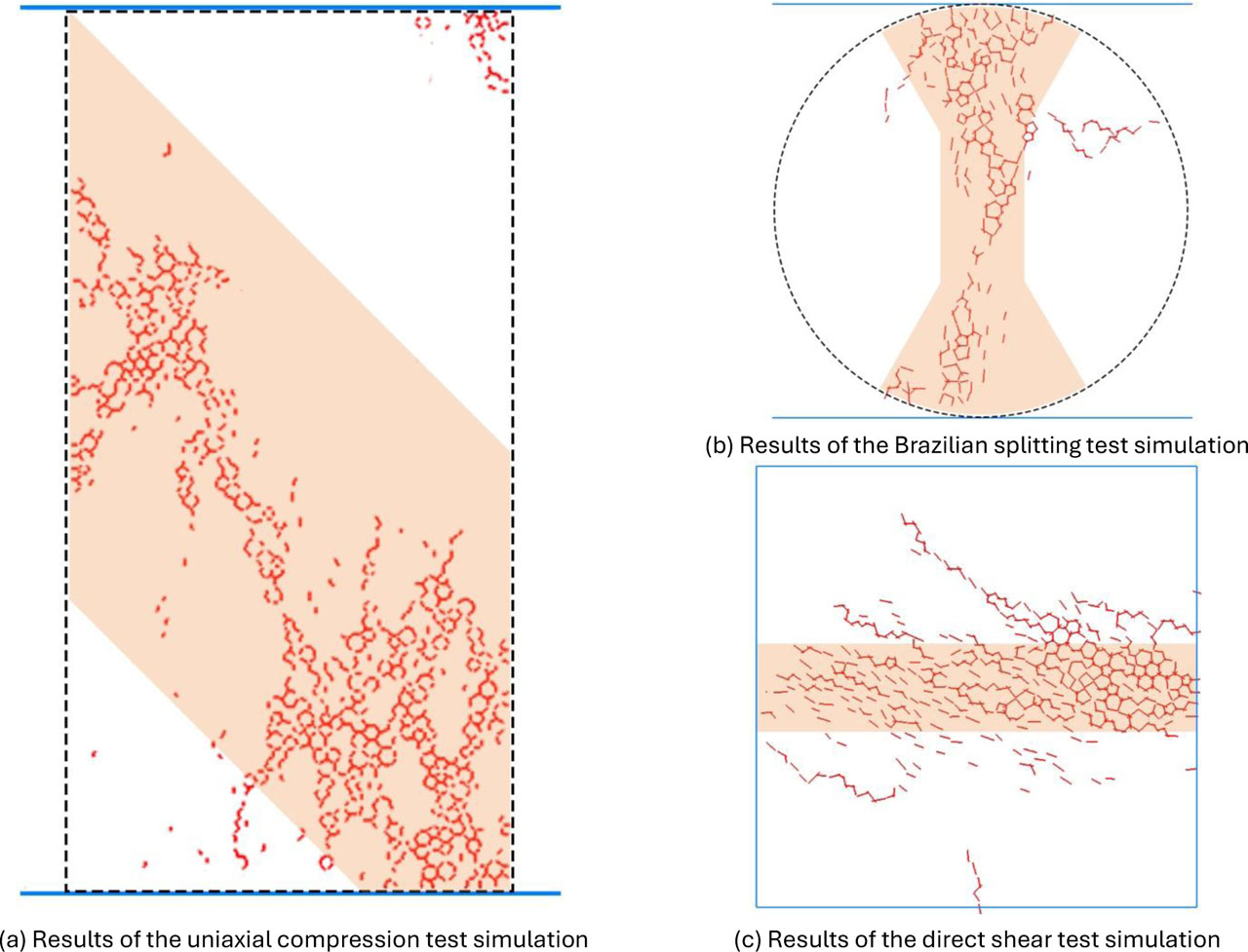
Figure 10:
Simulation results of the example rock model
In the simulation process of the uniaxial compression test, totally 840 fractures are generated, and 728 of them are located in the area shown in Figure 10 (a). Therefore, the fracture morphology is judged as declining one. In the Brazilian splitting test and direct shear test, totally 489 and 702 fractures are generated, and 441 and 552 fractures are located in the area shown in Figure 10 (b) and (c). In terms of the Brazilian splitting test results, the occupation of the generated fractures located in Figure 10 (b) is 0.90, which is higher than the criteria, and the fracture morphology is recorded as dumbbell, which is consistent with the K-nearest neighbors. However, in the direct shear test, the occupation of fractures in Figure (c) is only 0.79, so the fracture morphology is regarded as the large-scale one, which is different with the K-nearest neighbors method. Although the evaluating results differ with the simulation results, the occupation is extremely close to the criteria, which proves that the morphology of the example model has similarity of the linearly penetrated fracture morphology. The effectiveness of the evaluating method should be further verified by more numerical models with different micro-parameter combinations.
5. Results and Discussion
5.1. Verification results of the evaluation method
To verify the classification and evaluating method of the fracture morphology of the rock numerical model. Totally 40 combinations of the micro-parameter are uniformly and randomly generated in the range listed in Table 1, partial of which is shown in Table 7. In evaluating process, the k number of K-nearest neighbors is selected as 10, and the partial evaluating results of the 40 numerical model are listed in Table 8.
Table 7:
Micro-parameters of the partial of 40 randomly generated models used for verification
| σmi [MPa] | cmi [MPa] | λmi | ϕmi [°] | μmi | pmi | ||
|---|---|---|---|---|---|---|---|
| 1 | 72.54 | 79.27 | 0.81 | 34.29 | 57.15 | 0.75 | 0.14 |
| 2 | 23.17 | 33.43 | 0.93 | 87.36 | 40.08 | 0.29 | 0.12 |
| 3 | 27.46 | 82.32 | 0.68 | 39.38 | 53.93 | 0.89 | 0.12 |
| 4 | 68.40 | 80.92 | 0.81 | 44.96 | 44.54 | 0.19 | 0.12 |
| 5 | 13.54 | 10.54 | 0.93 | 12.98 | 41.54 | 0.24 | 0.13 |
| 6 | 89.82 | 46.19 | 0.56 | 66.44 | 48.51 | 0.31 | 0.10 |
| 7 | 51.20 | 39.16 | 0.62 | 73.92 | 49.74 | 0.76 | 0.11 |
| 8 | 40.58 | 50.71 | 0.73 | 48.10 | 47.27 | 0.56 | 0.14 |
| 9 | 17.39 | 31.60 | 0.62 | 27.31 | 50.19 | 0.51 | 0.13 |
| 10 | 22.46 | 33.27 | 0.63 | 29.81 | 47.42 | 0.34 | 0.15 |
| …… |
Table 8:
Partial Evaluating fracture morphology of the 40 verification models
| Uniaxial compression test | Brazilian splitting test | Direct shear test | |
|---|---|---|---|
| 1 | Declining | Dumbbell | Linearly penetrated |
| 2 | Declining | Large-scale | Linearly penetrated |
| 3 | Localized | Dumbbell | Linearly penetrated |
| 4 | Declining | Linearly penetrated | Linearly penetrated |
| 5 | Large-scale | Large-scale | Large-scale |
| 6 | Declining | Linearly penetrated | Linearly penetrated |
| 7 | Declining | Dumbbell | Linearly penetrated |
| 8 | Declining | Linearly penetrated | Linearly penetrated |
| 9 | Large-scale | Linearly penetrated | Large-scale |
| 10 | Declining | Large-scale | Large-scale |
40 numerical models are established by the combinations of the micro-parameters listed in Table 7, and the simulation of the test is conducted. Among them, partial simulation results are shown in Figure 11–13.
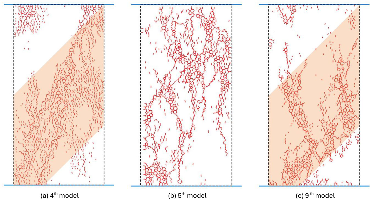
Figure 11:
The uniaxial compression test simulation results of partial verification models
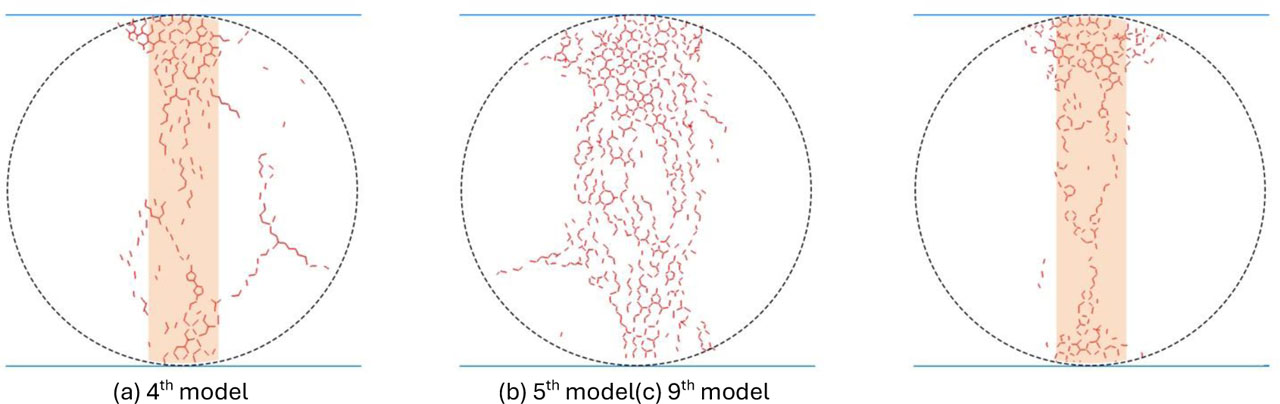
Figure 12:
The Brazilian splitting test simulation results of partial verification models
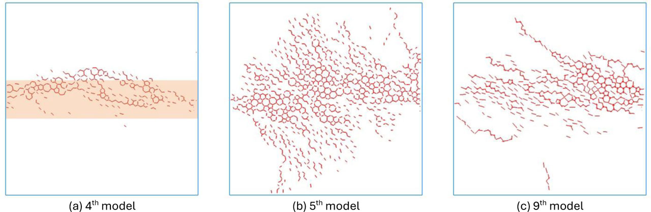
Figure 13:
The direct shear test simulation results of partial verification models
As Figure 11(a) shows, during the uniaxial compression test by the 4th model, there are totally 1573 fractures generated, and 1290 fractures are located in the orange area. Therefore, the fracture morphology generated in uniaxial compression test of the model is recorded as declining morphology. Similarly, the fracture morphologies of all models are recorded and shown in Figure 11–13. These simulated morphologies are compared with the evaluated results, as Figure 14 shows.
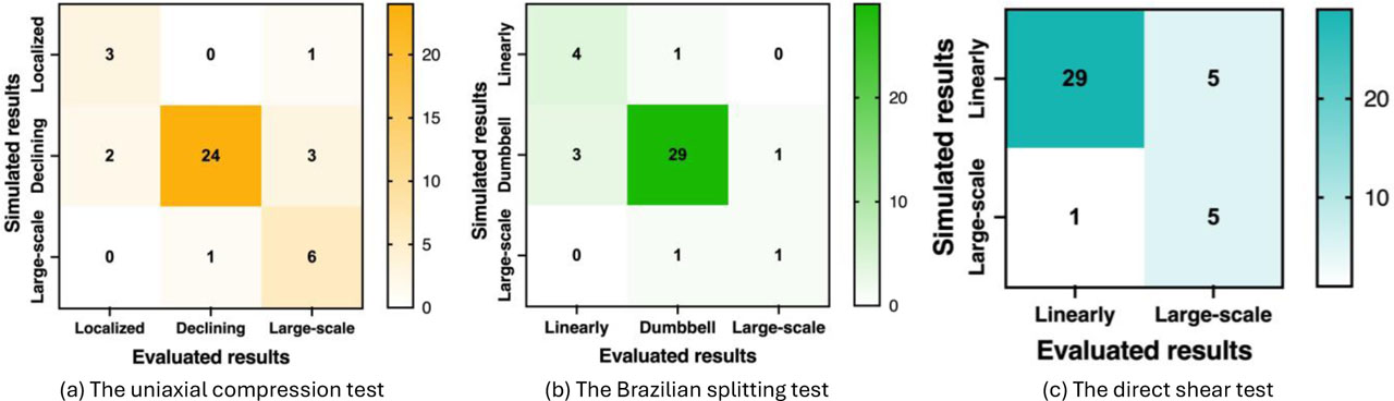
Figure 14:
Frequency of the comparison results between simulated and evaluated morphology
In Figure 14 (a)–(c), the horizontal and vertical axis represent the evaluated and simulated fracture morphology, and the color of the cubes represent the frequency of each kind of sample. In these figures, the cube located on the diagonal line from the top left to the bottom right represents the frequency of the sample with corrected evaluated results. There are totally 33, 34, and 34 corrected samples appeared in the three kinds of rock test, and the corresponding accurate rate reaches 82.5%, 85%, and 85%. Further, the precision and recall of the totally 8 kinds of fracture morphologies are listed in Table 9.
Table 9:
Statistic results of the evaluation method applied on the 40 added simulation
| Uniaxial compression test | Brazilian splitting test | Direct shear test | ||||||
|---|---|---|---|---|---|---|---|---|
| Localized | Declining | Large-scale | Linearly | Dumbbell | Large-scale | Linearly | Large-scale | |
| Precision [%] | 60.0 | 96.0 | 60.0 | 57.1 | 93.5 | 50.0 | 96.70 | 50.0 |
| Recall [%] | 75.0 | 82.8 | 85.7 | 80.0 | 87.9 | 50.0 | 85.30 | 83.3 |
| F1-score | 0.67 | 0.89 | 0.71 | 0.67 | 0.91 | 0.5 | 0.91 | 0.62 |
As Table 9 shows, the evaluated precision and recall is relatively acceptable. Except the Large-scale morphology in Brazilian splitting test and direct shear test, which might be affected by the small sample size, nearly all the precision and recall are higher than 60%. In terms of the main morphology with large sample size, such as the Declining morphology in uniaxial compression test, the Dumbbell morphology in Brazilian splitting test, and the Linearly morphology in direct shear test, the precision and recall are higher than 80%, and the corresponding F1-score is 0.89, 0.91, and 0.91. The average F1-score reaches 0.73. It proves that the evaluation results balance precision and recall, and the evaluation performance of the method is relatively good.
5.2. Comparison between multiple algorithm
On the basis of the proposed constraints of the fracture morphology, a fracture morphology evaluation method is developed by KNN, and the evaluation results are proved to be accurate and acceptable. In order to further verify the reliability of KNN on the dataset, the other classifiers, including support vector machine (SVM) and artificial neural networks (ANN) are tried to solve the same dataset. The two classifiers are achieved in Weka 3.6.1. Toally 1517 samples introduced in Section 2 is used as the training set, and the 40 simulation samples introduced in Section 5.1 is used as the testing set. By error- and trail, a series of hyper-parameters of SVM and ANN is selected, and the testing results is shown as Figure 15, and the corresponding precision and recall are listed in Table 10.
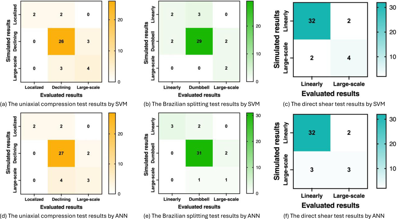
Figure 15:
Evaluating results of SVM and ANN
Table 10:
Statistic of the evaluated results by SVM and ANN
| Uniaxial compression test | Brazilian splitting test | Direct shear test | |||||||
|---|---|---|---|---|---|---|---|---|---|
| Localized | Declining | Large-scale | Linearly | Dumbbell | Large-scale | Linearly | Large-scale | ||
| SVM | Precision [%] | 100.0 | 83.4 | 57.1 | 50.0 | 90.6 | 50.0 | 94.1 | 67.0 |
| Recall [%] | 50.0 | 89.7 | 57.1 | 40.0 | 87.9 | 100.0 | 94.1 | 66.7 | |
| F1-score | 0.67 | 0.86 | 0.57 | 0.44 | 0.89 | 0.67 | 0.94 | 0.67 | |
| ANN | Precision [%] | 100.0 | 81.8 | 60.0 | 100.0 | 91.2 | 33.0 | 91.4 | 50.0 |
| Recall [%] | 50.0 | 93.10 | 42.9 | 60.0 | 93.9 | 50.0 | 94.1 | 60.0 | |
| F1-score | 0.67 | 0.87 | 0.50 | 0.75 | 0.93 | 0.40 | 0.93 | 0.55 | |
As Figure 15 shows, the evaluated results by SVM and ANN is also acceptable, as the darkest color appeared on the diagonal line from the top left to the bottom right, which means the correct evaluated results are given by SVM and ANN for most of samples. In terms of the three kinds of tests, there are 32, 33, and 36 correct results are given by SVM, and 32, 34, and 35 correct results are given by ANN. On the whole, the evaluation accuracies of SVM and ANN are closed to the one of KNN.
As Table 10 shows, the average F1-scores of SVM and ANN are 0.71 and 0.70, respectively, which is also closed to the level of KNN. However, there is a significant imbalance of the precision and recall of SVM and ANN. There are 6 and 5 precision or recall values lower than 0.60 appear in the results of SVM and ANN, which is only 3 values of KNN, while the lowest precision or recall of SVM and ANN is 40.0% and 33.0%, which is 50.0% of KNN. According to Figure 15, the evaluated results by SVM and ANN tend to cluster towards the majority of samples, which is also the reason of the imbalance of SVM and ANN results. Therefore, although the accuracy of SVM and ANN keeps similar level of KNN, considering the imbalance of the evaluated results, KNN is the most suitable algorithm to evaluate the generated fracture morphology.
The reason for the results is speculated to be that the SVM and ANN are suitable for solving the strongly nonlinear and complex problem by small size of samples. In this research, the generated fracture morphology is closely related to the micro-parameters, and the generated fracture morphologies of the numerical models constructed by similar micro-parameter combinations are hardly to exhibit significant differences. In addition, there is only two or three groups are set for each kind of rock test in this research, which also results in the nonlinearity and complexity of this problem is slightly weaker than conventional classification problem in the field of engineering geology. In other words, simple and direct classification method, such as KNN, is more suitable for evaluating generated fracture morphology than methods with high complexity.
5.3. Discussion
This section mainly discusses the potential and limitation of this research.
1. Potential
This research is mainly aiming at the fracture morphologies generated in the numerical simulation process of the different rock test, by using numerical models with different micro-parameter combinations. In geotechnical engineering, the macro-parameters, such as the uniaxial compressive strength and tensile strength are used to describe the rock properties. However, in numerical simulation, the rock materials are defined by micro-parameters, part of which are listed in Table 1, instead of the macro-parameters. Therefore, during building numerical models, an accurate relationship between micro-parameters and macro-parameters should be established. In terms of a numerical model with known macro-parameters, the selection of micro-parameters is always not unique, which means that there are usually more than one micro-parameter combinations meet the requirement of the model strength, and they should be screened. Especially, the fracture morphology generated in the rock test is an available filter to suppress the non-uniqueness of the micro-parameter combinations.
Take a field rock sample came from a bridge project in Southwest China as an example, its uniaxial compressive strength tested by the uniaxial compression test is 84.0 MPa, and its broken photo is shown as Figure 16. According to its compressive strength, 10 micro-parameter combinations with the uniaxial compressive strength error lower than 5%, also the uniaxial compressive strength ranges from 79.8MPa to 88.2MPa are randomly selected among the 1517 samples. The errors between the actual strength and the simulated strength of each selected sample are lower than 5%. In terms of the compressive strength, all of the combinations listed in Table 11 meet the requirement. In fact, part of the simulated fracture morphologies are not matched the actual test results.
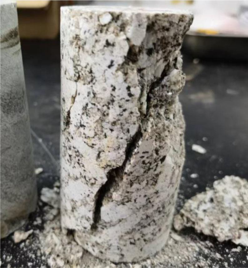
Figure 16:
Broken photo of the field rock sample
Table 11:
The micro-parameters of the selected samples
| σmi [MPa] | cmi [MPa] | λmi | ϕmi [°] | μmi | pmi | Morphology | ||
|---|---|---|---|---|---|---|---|---|
| 1 | 29.04 | 75.33 | 0.97 | 18.82 | 51.82 | 0.44 | 0.13 | Declining |
| 2 | 61.17 | 30.16 | 0.87 | 77.71 | 52.14 | 0.80 | 0.13 | Large-scale |
| 3 | 63.29 | 33.45 | 0.78 | 60.39 | 41.95 | 0.23 | 0.12 | Declining |
| 4 | 78.89 | 35.12 | 0.92 | 70.39 | 58.92 | 0.31 | 0.12 | Declining |
| 5 | 65.17 | 28.22 | 0.92 | 85.61 | 48.28 | 0.29 | 0.12 | Large-scale |
| 6 | 58.47 | 67.00 | 0.53 | 24.55 | 50.73 | 0.40 | 0.10 | Declining |
| 7 | 52.55 | 29.80 | 0.68 | 26.13 | 41.89 | 0.67 | 0.11 | Large-scale |
| 8 | 26.12 | 33.79 | 0.97 | 73.89 | 51.69 | 0.65 | 0.11 | Declining |
| 9 | 72.77 | 36.09 | 0.90 | 34.68 | 59.95 | 0.66 | 0.10 | Declining |
| 10 | 45.59 | 29.63 | 0.94 | 35.86 | 54.30 | 0.78 | 0.13 | Large-scale |
According to the proposed classification of the morphologies, the morphology of the actual sample is declining one, and only 1#, 3#, 4#, 6#, 8#, and 9# meet the requirement. The rest of the listed combinations cannot accurately reflect the rock behavior in the test, and they should be excluded from the selection for establishing the numerical model. The fracture morphologies generated in the Brazilian splitting test and the direct shear test can also be used as the basis to reduce the selection area of the micro-parameters to suppress their non-uniqueness.
2. Limitation
This paper investigated the effect of the micro-parameters of the numerical model on the fracture morphologies generated in several common rock test, and method for evaluating the fracture morphology is proposed. However, there is still several limitations of the method.
This research is conducted on the basis of simulation results of the totally 1517 numerical models with different micro-parameters. However, the ranges of the micro-parameters are limited by the limited computing resources. In fact, there are significant differences of the micro-parameters of different rock material. In terms of the rock with the micro-parameters outside the ranges shown in Table 1, the generated fracture morphologies may not be accurately evaluated by the proposed method. More simulations with extended micro-parameters ranges should be conducted in the futural studies.
In this research, the fractures generated by rock test need to be classified, and it need to determine the spatial distribution area of each kind of morphology and a criteria coefficient k. In this paper, the area is given as Figure 7, and the coefficient is selected as 0.8. However, these selections are subjective and empirical and can be used as a reference. During the actual simulation process, the area and coefficient should be further adjusted.
According to the previous research and the simulation process, there are multiple factors beyond micro-parameter affecting the generated fracture morphology. In fact, the stoppage time node of the simulation has significant influence of the fracture morphology. Take one of the 1517 models with the uniaxial compressive strength of 84MPa as an example, the generated fractures in different time is shown as Figure 17.
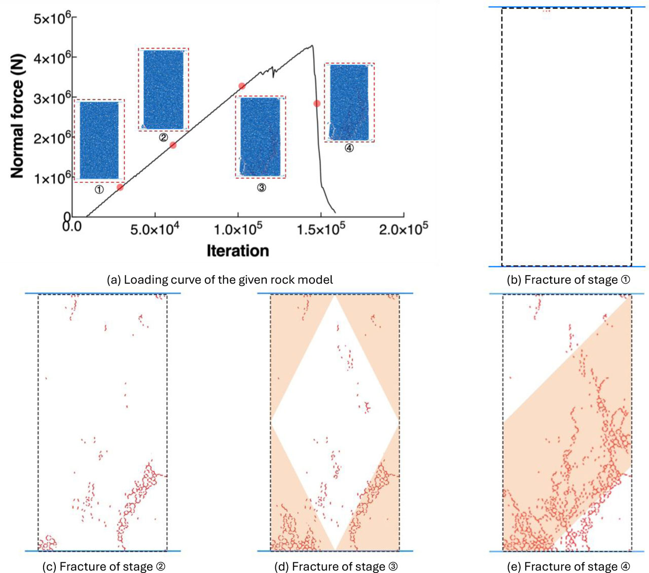
Figure 17:
The generating and extending process of the fractures in the uniaxial compression test
As Figure 17 shows, the fracture number increases with the increasing of the iterations. In the 1st and 2nd stage corresponding to the Figure 17 (b) and (c), the generated fractures are not penetrated the rock sample, and there are no fragments peeled off the model. With the conducting of iteration, in the 3rd stage corresponding to the Figure 17(d), numbers of fractures are generated in the lower left and lower right corner, and some particles are peeled off the model. Correspondingly, there is a significant fluctuation appeared on the load curve near the 3rd stage, shown in Figure 17(a). Also as shown in Figure 17 (d), if the simulation is ended near this stage, the morphologies of this sample might be judged as the localized one. In fact, the load is continuously increasing, and numbers of fractures appeared in the center area of the model in the 4th stage, as shown in Figure 17 (e). Accordingly, the morphology of this model in the uniaxial compression test are recorded as the declining one.
The example indicates that with the different ending criterion, the recorded fracture morphologies might be different. Especially, a universal and automatic ending criterion is used in this research, because there are numbers of models are used in simulation. In this research, the axial load is used as the ending criterion, i.e. when the current load decreased to be lower than the maximum of the historical load, the simulation should be ended. This criterion achieved acceptable results in the used 1517 models. However, the criterion is still subjective and empirical, and may not be applied to every rock numerical model. It also results in the fracture morphology results of some original models, which are not matched with the actual results. By conducting more rock test simulation to proposed a more reasonable ending criterion, is one of significant works in the futural research.
6. Conclusion
The main conclusion of this paper is summarized as follow.
Totally 1517 numerical models with different micro-parameters are established, and they are used to simulate the uniaxial compression test, Brazilian splitting test, and direct shear test. According to the distribution of the generated fractures, a classification method of the fracture morphology is proposed. The morphology generated in the uniaxial compression test is divided into three groups, including localized, declining, and large-scale morphology. The morphology generated in the Brazilian splitting test is divided into three groups, including linearly penetrated, dumbbell, and large-scale morphology. In addition, the morphology generated in the direct shear test is divided into two groups, including linearly penetrated and large-scale morphology.
It is found that the micro-parameters of the numerical models have significant influencing on the generated fracture morphology. In the uniaxial compression test, the localized fracture morphology mainly appears on the numerical model with high cohesion strength and low tensile strength, while the large-scale morphology mainly appears on the model with low tensile strength. In the Brazilian splitting test, the dumbbell morphology mainly appears on models with high friction coefficient, and large-scale morphologies are always with low cohesion strength, tensile strength, or effective module.
According to the simulation data and the fracture classification, a method for evaluating the fracture morphology based on the K-nearest neighbors is proposed. Based on the known micro-parameters of a numerical model, models with similar micro-parameters among the 1517 samples are searched, and the most possibly appeared morphology in uniaxial compression test, Brazilian splitting test, and the direct shear test is given as the evaluating results. To verify the method, 40 numerical models with random micro-parameter combinations are evaluated by the proposed method and compared with the actual simulated results. The accuracy in the uniaxial compression test and Brazilian splitting test is 82.5%, and the accuracy in the direct shear test reaches 85%. It proves that the method is acceptable and accurate. This method can evaluate the generated fracture morphology before simulating, and save the time cost in the trail-and-error during micro-parameters calibration. In addition, the method has potential on suppression the non-uniqueness of the micro-parameter combination, and it is helpful for establishing accurate and reasonable numerical model.
Acknowledgements
The research was supported by the Natural Science Foundation of Shandong Province (No. ZR2024QE150), and Postdoctoral Innovation Program Project of Shandong Province (No. SDCX-ZG-202503076).
Notes
[1] Contributed by Author Contributions
L.Z. acquired the funding and conducted the simulation of this study. R.W. acquired the funding, proposed the method, and wrote the original manuscript. B.L. conducted the filed investigation. J.H. conducting the simulation and wrote the original manuscript. N.L. conducting the simulation and wrote the original manuscript. All authors critically reviewed and approved the final version of the manuscript and agreed to be accountable for all aspects of the work.