
Recent changes in global climate have occurred more rapidly than previously anticipated, with increasing surface temperatures and enhanced climate variability observed across many regions (Beaugrand et al., 2025; Hansen et al., 2025). While global mean surface temperatures have risen by approximately 0.8°C to 0.9°C since the 1980s, recent observational data indicates that the warming rate has accelerated from 0.18°C per decade (1970–2010) to nearly 0.30°C per decade in the post-2010 period (Forster et al., 2025). This rapid escalation is primarily driven by the sustained accumulation of anthropogenic greenhouse gases, further compounded by a significant reduction in the cooling effect of sulphate aerosols (Hansen et al., 2025). In addition to temperature changes, global precipitation patterns have also shifted, with increasing trends observed in many tropical regions and decreasing trends in parts of the subtropics and mid latitudes (Gu & Adler, 2018; Nazeri Tahroudi, 2025). These changes have intensified the occurrence of extreme events such as floods (A. Ahmed et al., 2022; Fofana et al., 2022) and droughts in recent decades (Ha et al., 2022; Tripathy et al., 2023). Such developments highlight the urgent need for effective climate mitigation and adaptation strategies supported by reliable climate projections (Ouyang et al., 2025).
Climate projections are commonly derived from the Coupled Model Intercomparison Project, a coordinated framework that facilitates the comparison of global climate models developed by research institutions worldwide (Eyring et al., 2016). The most recent phase, CMIP6, provides simulations under the Shared Socioeconomic Pathways that integrate greenhouse gas emission trajectories with socioeconomic development scenarios (Riahi et al., 2017). These simulations have been widely used in climate change impact assessments at global and regional scales (Gebrechorkos et al., 2023; Gutowski Jr. et al., 2016; Tebaldi et al., 2021). However, the performance of CMIP6 models varies substantially across regions and climate variables, particularly in regions with complex atmospheric and oceanic interactions such as Southeast Asia (Khadka et al., 2022; Ngo-Duc et al., 2024). Therefore, systematic evaluation of model performance against historical observations is essential before applying these datasets to impact studies (Wagener et al., 2022).
The importance of accurate climate model evaluation is further underscored by its direct implications for hazard risk assessment and adaptation planning. Studies in Southeast Asia have demonstrated that precipitation projections from downscaled climate models serve as the primary input for projecting future flood and drought occurrence at the basin scale, where errors in simulated precipitation propagate directly into hydrological risk estimates (Voon et al., 2022). In Indonesia specifically, precipitation intensity is also closely linked to slope instability and landslide hazard, particularly in mountainous regions where high rainfall rates trigger slope failure (Nofrizal et al., 2025). These downstream applications make it critical that the GCMs used as forcing data adequately represent the spatial and temporal characteristics of precipitation, reinforcing the need for rigorous multi-metric evaluation prior to any regional application.
Evaluating climate model performance is inherently challenging because models must reproduce mean climate states, spatial patterns, temporal variability, and error magnitude across multiple scales (Eyring et al., 2019; Karpasitis et al., 2025). Numerous statistical metrics have been developed to quantify different aspects of model skill, including correlation based (Taylor, 2001), variability based (Gupta et al., 2009), and error-based measures (Legates & McCabe, 1999). Reliance on a single metric may lead to misleading conclusions, as a model may perform well according to one criterion while performing poorly according to another. Consequently, multi metric evaluation frameworks have gained increasing attention as a means to provide a more comprehensive assessment of model performance (Eyring et al., 2019).
Despite the growing number of CMIP6 evaluations, relatively few studies have applied integrative frameworks that combine multiple performance metrics into a single diagnostic measure (Akinsanola et al., 2021; Desmet & Ngo-Duc, 2022). Many previous studies focus on individual metrics or specific climate variables, often overlooking the integration between spatial, temporal, and statistical dimensions of model performance. To address this limitation, this study applies the Bergen Metrics framework, which integrates multiple evaluation metrics using Euclidean distance (Samantaray et al., 2024). This approach offers the advantage of simultaneously accounting for spatial, temporal, and magnitude-based performance in a transparent and reproducible manner. However, it carries an inherent limitation in that equal weighting is assigned to all constituent metrics by default, which may not reflect the relative importance of each metric for specific applications, and the Euclidean distance measure is sensitive to the scaling of individual metrics.
The objective of this study is to evaluate the performance of six CMIP6 models over Indonesia using the SA-OBS observational dataset. Model skills are assessed for precipitation, minimum temperature, mean temperature, and maximum temperature using five complementary metrics. The results are synthesized using Bergen Metrics and compared with a rank based weighting approach to identify robust model performance patterns. This study aims to support informed model selection for regional climate analysis, downscaling, and impact assessment.
Indonesia is situated in the maritime continent, spanning approximately 95°E to 141°E longitude and 6°N to 11°S latitude, making it one of the most climatically complex regions in the world. The country consists of over 17,000 islands encompassing a total land area of roughly 1.9 million km2, with the five major islands of Sumatra, Java, Kalimantan, Sulawesi, and Papua accounting for most of its landmass. Its equatorial position subjects the entire archipelago to a tropical climate characterized by high temperatures, high humidity, and abundant rainfall throughout the year. Mean annual temperatures generally range between 25°C and 28°C at low elevations, with limited seasonal variation in temperature but pronounced seasonality in precipitation driven by the Asian-Australian monsoon system. The northwest monsoon (November to March) brings wet conditions across much of the western archipelago, while the southeast monsoon (May to September) introduces drier conditions, particularly over Java, Bali, and the Lesser Sunda Islands (Aldrian & Dwi Susanto, 2003). This contrasting monsoon regime creates a strong west–east gradient in rainfall seasonality across the archipelago.

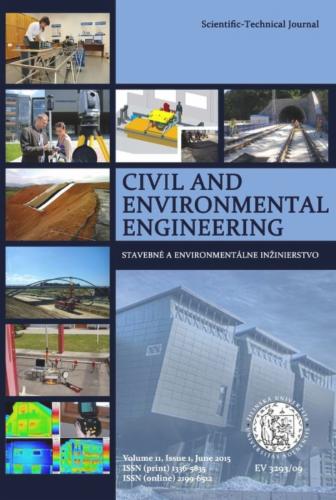
Topographic map of Indonesia and surrounding countries
Topography plays a critical role in shaping Indonesia’s climate shown on Figure 1, particularly for precipitation and temperature distributions. The terrain is highly heterogeneous, with several mountain ranges exceeding 4,000 meters above sea level, most notably in Papua where Puncak Jaya reaches approximately 4600 m. The orographic effect of these mountain ranges enhances convective precipitation on windward slopes and creates rain shadows on leeward sides, resulting in substantial spatial variability in rainfall at sub-regional scales. The complex land–sea configuration, extensive coastlines, and the presence of numerous narrow straits further amplify mesoscale convective systems and sea breeze circulations, which contribute significantly to local precipitation patterns. These physiographic characteristics pose inherent challenges for global climate models, whose coarse horizontal resolutions are often insufficient to resolve the fine-scale topographic and coastal features that govern Indonesia’s climate variability. Understanding this geographical and climatic context is therefore essential for interpreting the model evaluation results presented in this study.
The CMIP6 models were gathered from Earth System Grid Federation (https://esgf.nci.org.au/search), from 1981 to 2014, listed on Table 1. The selected CMIP6 models were chosen based on several evaluation studies over Southeast Asia (Desmet & Ngo-Duc, 2022; Moise et al., 2024; Nguyen et al., 2024). Daily dataset was used for precipitation (pr), average near-surface air temperature (tg), maximum near-surface air temperature (tx), and minimum near-surface air temperature (tn). These variables were chosen due to the observation of past study over Indonesia across three decades, which revealed changes in extreme temperature and precipitation and as indicator for tracking climate change in the region. All of the datasets then remapped using Climate Data Operators (CDO) (Uwe, 2023), remapcon for precipitation and remapbil for temperatures, into 0.25° horizontal resolution. The methods were based on how the variable behave: temperature is mostly continuous, so bilinear interpolation is the most suitable and as precipitation is representing amount over an area, so conservative remapping is suitable to preserve the statistics (Diaconescu et al., 2015). The same tool was also used to calculate each metric, using the default function and customized equation. The models then were compared with the observation dataset from SA-OBS (van den Besselaar et al., 2017), which provide gridded observational dataset based on several meteorological stations across the Southeast Asia. The SA-OBS has finer horizontal resolution at 0.25°, compared to CRU-TS at 0.5° and limited temporal resolution at monthly basis (Harris et al., 2020).
List of global climate model dataset
| No. | Institution | Model | Horizontal Resolution |
|---|---|---|---|
| 1 | Common wealth Scientific and Industrial Research Organisation (CSIRO), Australia (Dix et al., 2019) | ACCESS-CM2 | ∼1.875° × 1.25° (192 × 144 grid) |
| 2 | Centre National de Recherches Meteorologiques (CNRM), France (Voldoire, 2019) | CNRM-CM6-HR | ∼0.5° (720 × 360 grid) |
| 3 | EC-Earth Consortium ((EC-Earth), 2019a) | EC-Earth3 | ∼0.7° (512 × 256 grid) |
| 4 | EC-Earth Consortium ((EC-Earth), 2019b) | EC-Earth3-Veg | ∼0.7° (512 × 256 grid) |
| 5 | Met Office Hadley Centre, United Kingdom (Ridley et al., 2019) | HadGEM3-GC31-MM | ∼0.83° (432 × 324 grid) |
| 6 | Max Planck Institute for Meteorology, Germany (Jungclaus et al., 2019) | MPI-ESM1-2-HR | ∼0.94° (384 × 192 grid) |
Taylor Skill Score (TSS) is used to measure the overall performance of the model in producing spatial pattern (Taylor, 2001). The TSS is calculated as:
Rm - the spatial correlation between simulation and observation,
R0 - the maximum correlation between simulation and observation,
σm and σo - the spatial standard deviation of simulation and observation respectively.
The ideal score is equal to 1, when there is a perfect spatial match between simulation and observation, and score equal to 0 means inverse model performance. TSS were calculated spatially and then averaged by temporal, to obtain a single score for each model.
Interannual Variability Score (IVS) is used to evaluate the temporal variability of the simulation against the observed (Scherrer, 2011). The IVS is calculated as:
STDm and STDo – the temporal standard deviation of simulation and observation, respectively.
IVS were calculated temporally for each grid and then spatially averaged to get a single score for each model.
Mean Absolute Error was used in this study to evaluate how far the error of the simulations against observation. MAE was chosen because it is better than Root Mean Squared Error in visualizing the error (Willmott & Matsuura, 2005). The MAE was normalized using observation’s standard deviation of each month of the entire timeline, using ymonstd in CDO.
MAE was calculated by averaging the difference or the error (ei) between simulation and observation and divided by the standard deviation (σo) of the observation. The decision to normalize the MAE was due to the difference in error between precipitation and temperatures. Thus, it can be compared to the performance between variables without such skewness. The ideal score is 0, which indicates no skew between simulations and observation, and extends to ∞. The MAE was calculated temporally for each grid and then averaged by its spatial.
Kling-Gupta Efficiency (KGE) is mostly used as a goodness indicator of a hydrological model, in this case is precipitation or rainfall data (Kling et al., 2012). Although it is a hydrological indicator, a study also used KGE to evaluate models in producing temperature data (Mohammadlou et al., 2022). The KGE used in this study was the revised version of the original KGE, and calculated as follows:
r – the temporal correlation between simulation and observation,
μm and μo - temporal averages of simulation and observation respectively,
σm and σo are temporal standard deviation of simulation and observation respectively.
According to Knoben et al. (2019) the value of KGE is not symmetrical, negative value does not necessarily mean bad performance. They argued that −0.41 < KGE ≤ 1 is considered good performance, if the mean flow KGE = 1 – √2 is used. The single score of KGE for each model was calculated the same as the MAE and IVS.
Willmott Index (WI) or Index of Agreement, measures how well the model’s predictions match the observed data (Willmott et al., 2012). Several studies used Willmott Index to measure climate model’s performance in generating meteorological variables (K. Ahmed et al., 2019; Vicente-Serrano et al., 2025). The Willmott Index used in this study was the refined version, which is shown below:
As stated in their study, the Willmott Index was calculated by temporal to better represent the score. Mi and Oi are the ith value of simulation and observation respectively. Ō is the average of the observation, which we calculated using ymonmean in CDO as opposed to averaging it by seasonal as their recommendation. By using monthly-year average, we could rectify the sensitivity of precipitation. Since Indonesia is a tropical country with only two seasons (dry and wet season), the observed variability of precipitation would be low as the yearly mean is high relative to the daily data. The suppression is also applied to the temperatures. Temperature variability in Indonesia is relatively stable, compared to the temperate regions. Thus, errors are highly sensitive in Willmott Index, as the observed variability would be low. As for the value of c, we used the recommended value c = 2. The same calculation of the single score of each model was used in this metric, same as KGE, MAE, and IVS.
To summarize the scoring system, we utilized Bergen Metrics (Samantaray et al., 2024). The calculations are entirely based on the ideal score for each metric, which measures the distance between ideal score and the actual score of said metrics. The equation is as follows:
The Bergen Metrics were calculated per variable, five metrics for each variable: (1) precipitation, (2) minimum temperature, (3) average temperature, and (4) maximum temperature. The p value used in this study is p = 2. The calculation follows this regiment: (ideal score – actual score). With exception if the ideal score is 0, then the calculation is (metrics)p. As for the final score, the Bergen Metrics for each variable then also calculated using Bergen Metrics.
In addition to the Bergen Metrics scoring, a rank-based weighting (RANK) approach was applied to generate model weights based on performance across all five-evaluation metrics. This method follows the framework of Chen et al. (2011) Chyba! Nenašiel sa žiaden zdroj odkazov. and was generalized here for TSS, IVS, nMAE, KGE, and WI. For each metric, all models were ranked from best to worst. Metrics where higher values indicate performance (TSS, KGE, WI) were ranked in descending order, whereas the other (IVS, nMAE) were ranked in ascending order. For each model i, the Total Rank Score (Si) is then calculated as the simple sum of its rank positions across all M metrics for a given variable:
The Total Rank Score (Si) is an error proxy, meaning a lower value indicates better performance. To transform this into a performance indicator where a higher value reflects better model skill, the score is calculated as the inverse of Si, normalized by the sum of all model rank scores. The resulting performance indicator, Ri, for a single variable is defined as:
N – the total number of models in the ensemble.
A higher value of Ri indicates superior model skill. To obtain a single, robust weight reflecting the model’s overall performance across all analyzed climate variables (V), the following steps were followed: (1) the indicator Ri was averaged across all V climate variables to yield the model’s mean performance score (RM), and then (2) the final weight (Wi) was derived by normalizing the mean performance score RM, ensuring the sum of all model weights equals unity.
The final weight Wi represents the fractional contribution of model i to the final weighted multi-model ensemble projection. A model assigned to a higher Wi value is deemed to have the highest overall skill in simulating historical climate.
All evaluated models demonstrate limited skill in simulating daily precipitation over Indonesia, as shown in Table 2. Taylor Skill Score values below 0.25 indicate weak spatial correspondence with observed rainfall patterns. Willmott Index values are positive for all models, indicating some agreement in precipitation magnitude, although the agreement remains weak. In contrast, Kling Gupta Efficiency values are negative across all models, indicating poor combined representation of mean state, variability, and temporal correlation.
Model’s performance on precipitation
| Model | TSS | IVS | nMAE | KGE | WI |
|---|---|---|---|---|---|
| ACCESS-CM2 | 0.212 | 0.716 | 1.231 | −0.564 | 0.168 |
| CNRM-CM6-1-HR | 0.210 | 0.855 | 1.185 | −0.588 | 0.213 |
| EC-Earth3 | 0.231 | 0.632 | 1.096 | −0.494 | 0.241 |
| EC-Earth3-Veg | 0.230 | 0.631 | 1.099 | −0.494 | 0.241 |
| HADGEM-GC31-MM | 0.184 | 1.092 | 1.191 | −0.449 | 0.225 |
| MPI-ESM1-2-HR | 0.235 | 1.261 | 0.972 | −0.331 | 0.303 |
Normalized Mean Absolute Error further highlights persistent absolute biases in precipitation simulations, even after normalization by monthly observational variability. MPI-ESM1-2-HR exhibits the lowest nMAE among the models, indicating relatively smaller average errors, followed by EC Earth3 and EC-Earth3-Veg. Nevertheless, performance in the precipitation remains weak overall.
The poor precipitation skill reflects the inability of global climate models to resolve mesoscale convection, complex coastlines, and strong land sea interactions that dominate rainfall processes over the Indonesian archipelago (Aslam, 2025; Love et al., 2011; Wei et al., 2020). Differences in convective parameterization schemes further contribute to inter model variability (Baba, 2020; HARA et al., 2009; Tost et al., 2006). Similar limitations in CMIP6 precipitation simulations over the Maritime Continent have been widely documented (Agiel et al., 2024; Hariadi et al., 2023; Moise et al., 2024).

Spatial mapping of IVS performance in precipitation
Based on Figure 2, the spatial distribution of the Interannual Variability Skill (IVS) is consistent with the previously discussed summary scores. All models show pronounced difficulty in reproducing interannual precipitation variability over Papua, where IVS values are generally high, indicating poor temporal skill. In contrast, Sulawesi exhibits the most favorable performance across models, followed by Borneo and Sumatra. Java also shows relatively weak temporal performance, although its IVS is consistently lower than that over Papua, suggesting moderately better representation of interannual variability.
A comparable spatial pattern is evident in Figure 3, which presents the normalized mean absolute error (nMAE). All models display large biases over Papua, reinforcing the indication of poor model performance in this region. However, Java shows the lowest bias among the major islands, which contrasts with its relatively weak IVS performance. This discrepancy suggests that, over Java, models can reproduce mean precipitation magnitudes more accurately, while still struggling to capture year to year variability. Across the remaining islands, model performance is broadly similar, although ACCESS-CM2 and CNRM-CM6-HR exhibit systematically larger biases than the other models.

Spatial mapping of nMAE performance in precipitation
Model performance improves substantially for minimum temperature relative to precipitation on Table 3. Moderate Taylor Skill Score values indicate that spatial patterns of minimum temperature are reasonably well captured. Interannual Variability Score values further indicate that year to year variability is reproduced with moderate skill.
Model’s performance at minimum temperature
| Model | TSS | IVS | nMAE | KGE | WI |
|---|---|---|---|---|---|
| ACCESS-CM2 | 0.392 | 0.558 | 3.748 | 0.001 | −0.392 |
| CNRM-CM6-1-HR | 0.681 | 0.587 | 2.497 | 0.005 | −0.211 |
| EC-Earth3 | 0.541 | 0.499 | 2.419 | 0.037 | −0.193 |
| EC-Earth3-Veg | 0.540 | 0.519 | 2.365 | 0.039 | −0.176 |
| HADGEM-GC31-MM | 0.560 | 0.548 | 2.615 | −0.084 | −0.224 |
| MPI-ESM1-2-HR | 0.431 | 0.586 | 2.648 | −0.010 | −0.197 |

Spatial mapping of IVS performance at minimum temperature
Despite this, Willmott Index values remain negative but close to zero, indicating limited agreement in magnitude. Kling Gupta Efficiency values range from slightly negative to near zero, suggesting small but persistent systematic biases. These results indicate that while models successfully capture the spatial distribution and temporal variability of minimum temperature, they struggle to reproduce the absolute magnitude accurately.
EC-Earth3-Veg and CNRM-CM6-HR achieve the lowest normalized Mean Absolute Error values and the best Bergen Metrics scores for minimum temperature, reflecting balanced spatial and temporal performance. Remaining biases are most evident in coastal and mountainous regions, where local surface processes influence nocturnal cooling (Fan et al., 2022; Nguyen-Duy et al., 2023; Zhang et al., 2024).
Based on Figure 4, the spatial distribution of the Interannual Variability Skill (IVS) for minimum temperature indicates substantially better temporal performance compared to precipitation across most regions. All models exhibit relatively low IVS values over Sumatra, Borneo, Sulawesi, and Java, suggesting that interannual variability in minimum temperature is generally well captured. In contrast to precipitation, poor IVS values are more spatially confined and appear primarily over Papua and parts of eastern Indonesia, where models still struggle to reproduce temporal variability.
Differences among models are more apparent in localized regions rather than at the island scale. EC-Earth3 and EC-Earth3-Veg show comparatively lower IVS over large portions of western Indonesia, whereas ACCESS-CM2 and CNRM-CM6-HR exhibit more spatial heterogeneity, with pockets of degraded skill, particularly over mountainous and coastal regions.

Spatial mapping of nMAE performance at minimum temperature
Figure 5 presents the normalized mean absolute error (nMAE) for minimum temperature and reveals a markedly different spatial behavior from IVS. While temporal variability is generally well represented, systematic biases remain widespread. All models display elevated nMAE over Papua and eastern Indonesia, indicating persistent magnitude errors in minimum temperature. Java and Sumatra show relatively lower biases, although nMAE values remain non-negligible, suggesting that accurate temporal variability does not necessarily imply accurate absolute temperature values.
Overall, the comparison between IVS and nMAE highlights that minimum temperature is more robustly simulated in terms of interannual variability than precipitation, but spatial biases in magnitude persist, particularly in regions with complex topography and land surface heterogeneity.
Mean temperature simulations exhibit consistent skill across all evaluated models, shown on Table 4. Taylor Skill Score values exceeding 0.5 indicate reasonable spatial agreement with observations, while Interannual Variability Score values show that year to year temperature fluctuations is well represented.
Model’s performance on average temperature
| Model | TSS | IVS | nMAE | KGE | WI |
|---|---|---|---|---|---|
| ACCESS-CM2 | 0.376 | 0.363 | 2.618 | 0.127 | −0.150 |
| CNRM-CM6-1-HR | 0.766 | 0.343 | 3.032 | 0.119 | −0.352 |
| EC-Earth3 | 0.577 | 0.643 | 2.635 | 0.078 | −0.259 |
| EC-Earth3-Veg | 0.574 | 0.645 | 2.554 | 0.083 | −0.241 |
| HADGEM-GC31-MM | 0.594 | 0.338 | 2.118 | −0.038 | −0.094 |
| MPI-ESM1-2-HR | 0.489 | 0.831 | 2.642 | 0.066 | −0.266 |
Kling Gupta Efficiency values are positive for all models, indicating satisfactory representation of mean state and variability. However, Willmott Index values remain negative, highlighting persistent magnitude bias. This combination indicates that models reproduce temporal structure and variability well but exhibit systematic offsets in absolute temperature values.

Spatial mapping of IVS performance in average temperature
The relatively small inter model spread reflects the dominance of large-scale radiative forcing in controlling mean temperature, making it easier to simulate than precipitation (Andrews et al., 2010; Yang et al., 2021). Systematic magnitude biases suggest that simple bias correction methods could substantially improve model performance for temperature-based applications.
Figure 6 shows the spatial distribution of the Interannual Variability Skill (IVS) for average temperature. Compared to precipitation and minimum temperature, average temperature exhibits the most spatially coherent and overall strongest temporal performance across all models. Low IVS values dominate over Sumatra, Borneo, Sulawesi, and Java, indicating that interannual variability in mean temperature is consistently well captured. Regions of degraded IVS are largely confined to Papua and parts of eastern Indonesia, where complex terrain and land–atmosphere interactions remain challenging for all models.
Model differences are relatively subtle for average temperature. EC-Earth3 and EC-Earth3-Veg tend to exhibit slightly lower IVS over western Indonesia, while ACCESS-CM2 and CNRM-CM6-HR show more localized variability, particularly over coastal and mountainous regions. Nevertheless, the inter-model spread in IVS is smaller than that observed for precipitation, suggesting greater robustness of average temperature simulations.

Spatial mapping of nMAE performance in average temperature
The normalized mean absolute error (nMAE) patterns shown in Figure 7 reveal that, despite strong temporal variability skill, substantial magnitude biases persist. All models display elevated nMAE over Papua, while Java and Sumatra consistently show lower biases. Like minimum temperature, this contrast indicates that accurate representation of interannual variability in average temperature does not necessarily translate into accurate absolute temperature values. MPI-ESM1.2-HR exhibits larger biases over several regions, particularly in eastern Indonesia, whereas EC-Earth3-based models generally show more spatially homogeneous errors.
Overall, average temperature emerges as the best simulated variable in terms of temporal variability, yet persistent spatial biases highlight the continued challenge of accurately representing mean temperature fields in regions with complex geography.
Maximum temperature is simulated with moderate skill across all models (Table 5). Taylor Skill Score values indicate reasonable spatial consistency and normalized Mean Absolute Error values remain relatively low. Kling Gupta Efficiency values suggest moderate efficiency with some model-dependent biases.
Model’s performance at maximum temperature
| Model | TSS | IVS | nMAE | KGE | WI |
|---|---|---|---|---|---|
| ACCESS-CM2 | 0.329 | 0.259 | 1.850 | 0.119 | −0.060 |
| CNRM-CM6-1-HR | 0.673 | 0.395 | 3.030 | 0.034 | −0.420 |
| EC-Earth3 | 0.499 | 0.436 | 2.466 | 0.094 | −0.273 |
| EC-Earth3-Veg | 0.495 | 0.442 | 2.388 | 0.101 | −0.252 |
| HADGEM-GC31-MM | 0.512 | 0.367 | 2.184 | −0.064 | −0.194 |
| MPI-ESM1-2-HR | 0.457 | 0.672 | 2.589 | 0.048 | −0.307 |

Spatial mapping of IVS performance at maximum temperature
Willmott Index values are negative for all models, although their magnitudes are small, indicating modest but consistent disagreement in magnitude. This pattern suggests that daytime heating processes are captured in relative terms, but systematic biases remain.
Differences in maximum temperature performance are likely related to the representation of surface radiation, cloud cover, and land surface energy balance processes (Lauer et al., 2023; Wang et al., 2023, 2025). Despite these limitations, temperature simulations remain substantially more reliable than precipitation simulations over Indonesia.
Figure 8 presents the spatial distribution of the Interannual Variability Skill (IVS) for maximum temperature. Overall, TX exhibits good temporal performance across much of western Indonesia, with low IVS values over Sumatra, Java, and large parts of Borneo and Sulawesi. This indicates that interannual variability in maximum temperature is generally well captured by all models. However, compared to average temperature, TX shows slightly higher spatial heterogeneity, particularly over coastal regions and areas influenced by strong land–sea thermal contrasts.

Spatial mapping of nMAE performance at maximum temperature
As with the other variables, Papua stands out as the region with the weakest IVS, where elevated values indicate persistent difficulty in reproducing year to year variability. This behavior is consistent across all models and mirrors the patterns observed for minimum and average temperature, underscoring the challenges associated with complex topography and land surface processes in eastern Indonesia. Among the models, EC-Earth3 and EC-Earth3-Veg display comparatively smoother IVS patterns, while ACCESS-CM2 and CNRM-CM6-HR show more localized regions of degraded skill. The normalized mean absolute error (nMAE) maps in Figure 9 reveal widespread and pronounced magnitude biases for maximum temperature. Compared to minimum and average temperature, TX exhibits the largest nMAE values across most regions, particularly over Sumatra, Borneo, and Papua. This indicates that, although temporal variability is reasonably well represented, models systematically misrepresent the magnitude of daily maximum temperatures. CNRM-CM6-HR and MPIESM1.2-HR show especially high biases over large areas, whereas EC-Earth3-based models exhibit relatively lower but still substantial errors.
In summary, maximum temperature demonstrates strong interannual variability skill comparable to other temperature variables, but it is the most biased in terms of absolute magnitude. This contrast highlights the sensitivity of TX to surface energy balance, cloud cover, and land–atmosphere coupling processes, which remain challenging to simulate accurately.
Integrated Bergen Metrics’ results, in Table 6, show that EC-Earth3-Veg achieves the lowest overall distance, followed closely by HadGEM3-GC31-MM and EC-Earth3. Models such as ACCESS-CM2 and CNRM-CM6-HR exhibit larger distances, indicating lower overall performance across variables.
Rank based weighting produces broadly consistent conclusions, with EC-Earth3-Veg and EC-Earth3 receiving the highest weights, displayed on Table 7. While Bergen Metrics accounts for metric magnitude through Euclidean distance, rank based weighting emphasizes relative consistency across metrics. The agreement between both approaches strengthens confidence in the identification of robust top performing models.
Bergen metrics on overall model’s performance
| Model | Precipitation | Minimum Temperature | Average Temperature | Maximum Temperature | BM |
|---|---|---|---|---|---|
| ACCESS-CM2 | 2.41 | 4.20 | 3.08 | 2.42 | 6.23 |
| CNRM-CM6-1-HR | 2.43 | 3.02 | 3.46 | 3.52 | 6.28 |
| EC-Earth3 | 2.24 | 2.94 | 3.16 | 2.99 | 5.71 |
| EC-Earth3-Veg | 2.24 | 2.90 | 3.08 | 2.92 | 5.61 |
| HADGEM-GC31-MM | 2.44 | 3.16 | 2.65 | 2.78 | 5.54 |
| MPI-ESM1-2-HR | 2.32 | 3.18 | 3.23 | 3.17 | 6.00 |
Rank-based weighting on overall model’s performance
| Model | Precipitation | Minimum temperature | Average temperature | Maximum temperature | RANK |
|---|---|---|---|---|---|
| ACCESS-CM2 | 4.38 | 4.04 | 7.00 | 10.50 | 0.161 |
| CNRM-CM6-1-HR | 4.38 | 6.18 | 6.18 | 5.00 | 0.135 |
| EC-Earth3 | 9.55 | 10.50 | 5.53 | 5.83 | 0.195 |
| EC-Earth3-Veg | 7.50 | 11.67 | 6.18 | 6.18 | 0.196 |
| HADGEM-GC31-MM | 4.77 | 5.25 | 9.55 | 7.50 | 0.168 |
| MPI-ESM1-2-HR | 10.50 | 4.57 | 4.04 | 4.20 | 0.145 |
The results of this study demonstrate that the choice of evaluation metrics strongly influences the interpretation of climate model performance. The combined use of spatial, temporal, and magnitude-based metrics reveals that CMIP6 models may reproduce spatial patterns and interannual variability well while still exhibiting systematic biases in absolute values. This is particularly evident for temperature variables, where relatively high Taylor Skill Score and Interannual Variability Score values coexist with negative Willmott Index values. Such behavior indicates that models correctly capture spatial gradients and temporal variability but suffer from consistent magnitude offsets, a characteristic commonly reported in global climate model evaluations (Bock et al., 2020; Krinner & Flanner, 2018; Schaller et al., 2011).
In this study, it was revealed that all the models demonstrated low performance of producing precipitation. All models scored low on spatial performance (TSS) and goodness-of-fit (KGE). Since both TSS and IVS used standard deviations, we could estimate the problem. IVS between 0.6 and 1.25 indicates that the ratio of standard deviations (simulation divided by observation) were either 0.585–0.68 or 1.47–1.7, which require the model to had at most spatial correlation of 0.1 to produce score 0.18 and 0.23 of spatial performance. Only MPI-ESM1-2-HR has KGE higher than the −0.41 threshold. This also translates the performance across TSS, nMAE, and WI that was the highest among all models, although it performed poorly on IVS. The poor performance of KGE might be due to the low spatial correlation of at most 0.1 and the nature of the variability in precipitation. A slight error in producing precipitation could heavily skew the ratio of standard deviation and ratio of average precipitation, which were used in KGE. As for the Willmott Index, the error was suppressed by the variability of the observation.
From all models and variables, the performance was elevation dependent, as shown on the spatial distribution of nMAE. For example, on maximum temperature, both EC-Earth3 and EC-Earth3-Veg performed better over mountainous areas of Sumatra, Java, Borneo, Sulawesi, and Papua. Similar results could also be observed for minimum and average temperatures. As for precipitation, all models overestimated Papua’s mountain range depicted in Figure 1, with pronounced wet biases along the central cordillera where orographic enhancement of rainfall is strongest and local convective processes are poorly represented at the native CMIP6 resolution (Lalande et al., 2021). This elevation-dependent overestimation implies that model skill assessed at the national or island-mean scale can conceal substantial regional errors, particularly over highlands that are critical for water resources and downstream hydrological impacts.
A further limitation of Bergen Metrics relates to its sensitivity to inter-model spread. The framework measures the Euclidean distance of each model from the ideal score, meaning that when all models perform similarly and their scores cluster closely together, the resulting distances may be numerically small and difficult to distinguish. Under such conditions, small differences in any single metric can disproportionately shift the overall ranking, reducing the reliability of the composite score as a discriminator. Samantaray et al. (2024) acknowledged that Bergen Metrics results should be interpreted alongside individual metric behavior rather than the composite score alone, precisely because the Euclidean distance is sensitive to how individual metrics resolve differences between models. This behavior contrasts with the rank-based weighting approach, which is inherently ordinal and always differentiates between models regardless of the absolute magnitude of performance differences, making it more robust when inter-model differences are small. This sensitivity to the choice of evaluation framework is broadly consistent with findings from other regions: Graff et al. (2025) demonstrated for Arctic climate storylines that no single performance score is universally applicable across all metrics and regions, and that model rankings shift depending on which variables are prioritized. A parallel pattern is evident in neighboring Peninsular Malaysia, where Sa’adi et al. (2026) found that the top-performing GCMs identified through an optimized multi-metric framework differed substantially from those selected using a single metric, with Pour et al. (2022) arriving at an entirely different set of recommended models when relying on KGE alone, underscoring that the choice of evaluation approach is itself a determinant of which models are deemed suitable for regional climate projections. Similarly, a multi-method comparison in southern Italy found that different ranking methods identified different best-performing models depending on the timescale of analysis, reinforcing that composite metrics should not be applied in isolation (Pellicone & Caloiero, 2025)Chyba! Záložka nie je definovaná.. Taken together, Bergen Metrics is most informative when the evaluated models show substantial spread in performance, and its results in this study should be interpreted with particular caution for temperature variables, where inter-model differences are small.
The application of Bergen Metrics in this study also introduces several limitations that are important to acknowledge when interpreting the integrated performance scores. First, the Euclidean distance formulation implicitly assumes that all standardized metrics contribute equally to the final score, so large systematic precipitation errors over key regions such as the Papua highlands can be partially compensated for by better performance in temperature or in other islands, leading to an overall distance that appears moderate despite serious regional deficiencies. Second, Bergen Metrics aggregates performance over space and variables without explicit regional weighting, which means that complex-terrain hotspots with strong elevation-dependent biases receive the same influence as relatively well-simulated lowland areas, even though they may be more relevant for impact-oriented applications such as flood risk or water resources planning. Third, the method is sensitive to the choice and scaling of the underlying metrics, so different combinations or normalizations of TSS, IVS, nMAE, KGE, and WI could yield different distances, adding a layer of subjectivity that is not always transparent to end users. In contrast, rank-based weighting emphasizes the relative ordering of models rather than the absolute magnitude of metric differences, which tends to preserve the identification of consistently poor precipitation performance—even when aggregated across variables – and can therefore offer a more robust perspective for model selection in regions with strong spatial heterogeneity such as the Papua mountain range.
This study evaluated the performance of six CMIP6 global climate models over Indonesia using a multi-metric framework synthesized through Bergen Metrics and complemented by a rank-based weighting approach. Overall, the results show that model skill is strongly variable across both variables and regions, with temperature fields being simulated more reliably than precipitation. Minimum, mean, and maximum temperatures exhibit reasonable spatial and temporal performance, although systematic magnitude biases persist, particularly over coastal and mountainous regions. In contrast, all models demonstrate limited skill in simulating daily precipitation, with low spatial correspondence, weak temporal variability, and large absolute errors. These deficiencies are most pronounced over the Papua mountain range, where complex topography and mesoscale convective processes lead to strong elevation-dependent overestimation that is not resolved at the native CMIP6 resolution.
The results reveal a consistent contrast in model suitability across climate variables. All evaluated models demonstrate limited skill in reproducing daily precipitation over Indonesia, with weak spatial correspondence and poor goodness-of-fit scores observed across the archipelago. This limitation is most pronounced over high-elevation regions such as Papua, where the complex terrain amplifies the inability of coarse-resolution global models to capture mesoscale convective processes and orographic rainfall. In contrast, temperature variables are simulated with considerably greater skill across all models, with average temperature exhibiting the strongest interannual variability performance and the most spatially coherent patterns. Minimum and maximum temperatures fall between these two extremes, showing reasonable spatial skill but persistent magnitude biases, particularly over elevated terrain. EC-Earth3-Veg emerges as the best overall performing model across all variables, followed by HadGEM3-GC31-MM and EC-Earth3, and is therefore most suitable for applications requiring a single model selection over Indonesia. The comparison between Bergen Metrics and rank-based weighting highlights that the choice of evaluation framework can substantially influence the interpretation of overall model performance. Bergen Metrics provides a compact and physically interpretable summary of multi-metric behavior, but its Euclidean aggregation can partially mask regional hotspots of poor performance when models compensate with better skill in other variables or regions. Rank-based weighting, on the other hand, is more sensitive to the relative ordering of models and tends to better preserve consistent weaknesses in precipitation, especially over complex terrain such as Papua. Taken together, the results emphasize that integrated model evaluation over Indonesia should not rely on a single metric or a single aggregation method. Instead, robust model selection for climate impact studies in the region should combine multi-metric synthesis, rank-based diagnostics, and region-specific analyses, with particular attention to high-risk areas where biases are elevation dependent and precipitation remains highly uncertain.