

1. Introduction
Piezoelectric is one of the most effective mechanisms in Structural Health Monitoring. This mechanism utilizes the piezoelectric effect, the ability of specific materials to generate electric charge when subjected to mechanical stress or deformation, and vice versa. The uniqueness of these electromechanical properties makes piezoelectric materials suitable for use as sensors and actuators (Aydin & Çelebi, 2023; Kim et al., 2024; Shaukat et al., 2023).
Ceramic and polymer, known as conventional piezoelectric materials, are suitable for application in steel structures, reinforcement, and masonry. Meanwhile, some studies have reported that these piezoelectric conventional systems are ineffective when applied to concrete structures (Ma et al., 2022).
The density of concrete (2.4 × 10³ kg/m3) as the host structure and piezoelectric materials (4.64 – 7.6 × 10³ kg/m3) as the sensor are significantly different. This condition causes the acoustic impedance mismatch, leading to the signal acceptance interference. During the hydration process, concrete experiences shrinkage and expansion; meanwhile, this change does not sync with the piezoelectric sensor. This condition results in partial loss of electric energy. Due to these reasons, piezoelectric materials are considered ineffective for application in concrete structures (Ding et al., 2021).
To overcome the acoustic impedance mismatch between concrete and piezoelectric materials, a cement-based piezoelectric composite (CPC) has been developed, combining cement as a base material for concrete with piezoelectric materials (Wu et al., 2022). Several connectivity patterns have been introduced for specific functions, primarily sensing and actuating in structural materials. The 0–3 connectivity type is the most widely used due to its ease of fabrication, good compatibility, homogeneous distribution, and its cost effectiveness (Ding et al., 2021; Pan et al., 2020; Sappati & Bhadra, 2018).
CPC is produced through a series of processes, including the most crucial and challenging step of polarization. This step involves immersing the CPC specimen into a silicon oil bath under a specific external electric field to align the electric dipoles. Polarization significantly influenced the quality of CPC, and the quality of polarization is significantly influenced by three factors: the external electric field, duration, and temperature. Studies have reported that higher levels of these factors lead to more effective polarization. However, the excessive levels can lead to the breakage of the specimen (Ding et al., 2021; Pan et al., 2020). High electric field (1–4 kV/mm) has been widely used and reported (Pan et al., 2020; Pan & Guan, 2022; Pan & Huang, 2020; Pan et al., 2019; Santos et al., 2020; Zhang et al., 2019); however, polarization under low electric field has promising potential. A low electric field can prevent dielectric breakdown and unwanted chemical reactions and can also produce a more controlled and homogenous polarization, making sensor performance more stable. A study conducted by Li et al. on 0–3 type CPC showed that the utilization of an electric field of 330 V/mm produced a piezoelectric strain (d33) of approximately 5 pC/N on day 180 (Li et al., 2005).
Electromechanical Impedance (EMI) Technique is a non-destructive method for observing the health and damage of materials or structures. Over the past two decades, piezoelectric-based EMI techniques have become one of the most widely used methods in SHM due to their cost-effectiveness, ease of signal interpretation, and high-frequency detection that allows for noise-free operation (Ai et al., 2024; Gedam & Khante, 2016; Wang et al., 2022). The inspected structural components are equipped with PZTs mounted on the surface or embedded within the concrete, and they are excited by an alternating voltage signal using an impedance analyzer or LCR meter with a specific frequency range (Jothi et al., 2017).
Several studies have reported the use of PZT-based EMI techniques in concrete structures. Gedam and Khante (2016) utilized thin PZT cast into mortar to assess the health and damage state of a reinforced concrete beam measuring 100 × 100 × 410 cm3 through susceptance and conductance signals recorded by the sensor (Gedam & Khante, 2016). Similarly, Jothi et al. (2017) employed PZT embedded in a concrete cube to evaluate the strength development during the early curing phase by analyzing the EMI signature, specifically the conductance signal (Jothi et al., 2017). Pan et al. (2019) used thin PZT and cement-based piezoelectric sensors to monitor the strength development of concrete cylinders over a period of 1 to 56 days. They also assessed the damage of reinforced concrete beams measuring 150 × 150 × 530 mm3 by recording the conductance signal (Pan et al., 2019). Pan and Huang (2020) further examined the development of compressive strength in 50 × 50 × 50 mm3 mortar cubes using PZT and cement-based piezoelectric sensors, as captured by impedance and conductance signals (Pan & Huang, 2020). Pan and Guang (2022) utilized PZT and CPC to observe the development of compressive strength, stress, and strain in cylindrical concrete at intervals of 1, 30, 60, and 90 days of age, as recorded by the conductance and impedance signals (Pan & Guan, 2022). Zhu et al. (2024) monitored the hydration of mortar blocks measuring 100 × 100 × 400 mm3 by embedding cement-based piezoelectric sensors within them. The relationship between conductance and hydration state was correlated (Zhu et al., 2024).
According to previous studies, polarization under low electric fields remains constrained to a maximum of 330 V/mm. Therefore, electric fields set at 250 V/mm and 375 V/mm show significant potential for development. Preliminary testing has indicated that polarization durations of 40 and 60 minutes give a higher piezoelectric strain coefficient (d33) compared to durations of 90 and 120 minutes. This study aims to assess the capability of CPC polarized under low electric fields in monitoring crack propagation within a mortar beam. Four variations are tested: C1 (250 V/mm for 40 minutes), C2 (250 V/mm for 60 minutes), C3 (375 V/mm for 40 minutes), and C4 (375 V/mm for 60 minutes). All sensors were embedded within the flexural area of beams measuring 100 mm × 100 mm × 400 mm3 and were subjected to flexural loads on day 28. The tests included assessments of spectrum conductance and beam strain under incremental loads until failure occurred. The performance of each sensor was evaluated by comparing the measured strain with the Root Mean Square Deviation (RMSD) of the conductance.
2. Methodology
2.1. Sensor Raw Materials
The Cement-based Piezoelectric Composite (CPC) sensor employed in this study was synthesized from a mixture of Lead Zirconate Titanate (PZT) crystal powder and Ordinary Portland Cement (OPC) with a volumetric ratio of 50:50. The OPC used has a density of 3.03 g/cm3. The PZT powder used was nano-sized, ranging from 100 to 150 nm, with a purity level of 99%. The PZT composition consists of 52 mol% Lead Zirconate (PbZrO3) and 48 mol% Lead Titanate (PbTiO3), with a density of 7.7 g/cm3. Based on several previous studies, PZT is known to have a high electromechanical coefficient and dielectric constant and is easily polarized, making it a very potential piezoelectric material for sensor applications. PZT is also the most used piezoelectric material in Structural Health Monitoring (SHM) systems (Aydin & Çelebi, 2023; Shaukat et al., 2023; Tiantong et al., 2022).
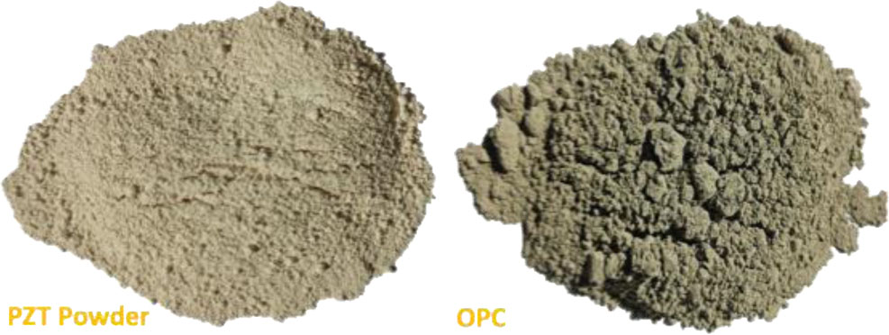
Figure 1:
Sensor raw material
2.2. Cement-based Piezoelectric Composites Fabrication Process
The homogeneous mixture of PZT powder and OPC, with a volumetric ratio 50:50 was cast into a steel mold. To produce a sensor with a diameter of 20 mm and a thickness of 2 mm, and a compact and strong mechanical structure, the mixture was compacted using a Universal Testing Machine (UTM) at a pressure of 80 MPa.
The disk-like sensor was cured at 90°C and 100% relative humidity for 24 hours. To reduce moisture and residue while preparing the sensor for the next stage, a pre-treatment process was carried out by heating the sensor in an oven at 140°C for 40 minutes. After this stage, the sensor surface and sides were polished to obtain a smooth and even texture. Both sides of the sensor surface are then coated with low-temperature silver paint to form active electrodes. After coating, the sensor undergoes a post-treatment process identical to the previous procedure to prepare for the polarization process (Ding et al., 2021). The heating process in the post-treatment stage is known to reduce the dielectric loss value, thus increasing the readiness of the specimen to undergo the polarization process (Pan et al., 2016, 2020).
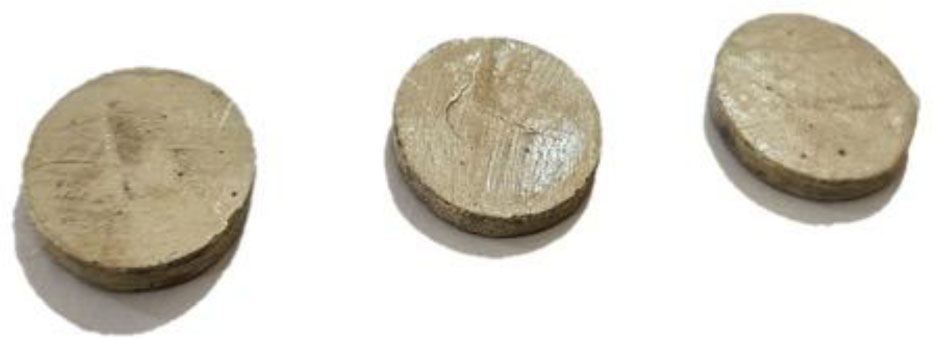
Figure 2:
The disk-like CPCs
Polarization is a crucial process in CPC sensor production, influenced by external electric fields, duration, and temperature. According to preliminary tests conducted previously, this study investigated polarization under low electric fields of 250 V/mm and 375 V/mm for 40 and 60 minutes. The selection of this electric field is due to the constraint that the use of a low electric field remains limited to 330 V/mm (Li et al., 2005). The sensor was immersed in a silicon oil bath and then treated according to the polarization conditions outlined in Table 1. After undergoing polarization, the sensors were stored in a Styrofoam box to preserve their polarized state.
2.3. Packaging of CPC and Mortar Beam
The CPC electrode surfaces were connected using copper foil as a conductive wire. To ensure insulation, half of the length of the copper foil was covered with a heat-shrinkable thermal casing. The sensor was then embedded within the cube of cement paste to protect it from potential damage during the casting process.
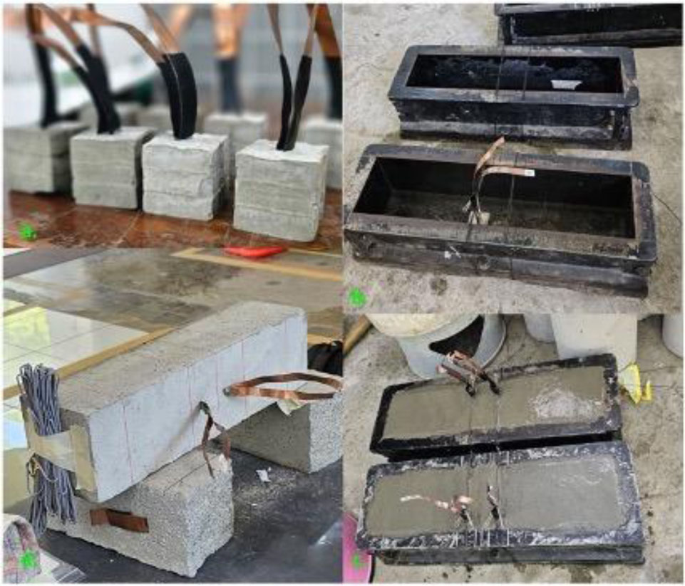
Figure 3:
Sensor and beam preparation
This study utilized a mortar beam (100 × 100 × 400 mm3) with a water-to-cement (w/c) ratio of 0,45. To maintain consistency in the data recorded by the sensor, two CPCs were embedded in the flexural area of the beam. Additionally, strain gauges were installed in the tensile area of the beam to measure strain during loading. Strain gauges were installed at position 1 cm, 2.5 cm, and 4 cm from the bottom of the beam. The packaging sensor and beam preparation are depicted in Figure 3. The positions of the CPCs and strain gauges are illustrated in Figure 4.
2.4. Experimental Monitoring of Beam Damage
A Study conducted by Al-Masraf et al. (2024) showed that the flexural loading condition significantly governs the initial and propagation crack in cementitious composites. This highlights the need to monitor what happens to a beam when it is bent (Al-Masraf et al., 2024). Similarly, Abed and Daud (2024) used a four-point bending test to assess the deterioration of corroded reinforced concrete beams under sustained loads. It also confirms that flexural testing is an established and reliable approach for evaluating damage evolution in concrete structures (Abed & Daud, 2024). In this research, a four-point bending test was used to create a pure bending region in the middle of the beam, where cracks are most likely to initiate. The difference is that, instead of only looking at the mechanical response, CPC sensors were embedded inside the mortar to track the electromechanical changes as damage developed directly. Crack propagations were carried out by subjecting the specimens to a series of incremental loads, ranging from 20% to 90% of the maximum bending load, until failure occurred. These load increments are specified in Table 2. All tests were conducted when the mortar was 28 days old to ensure optimal material maturity.
In this study, one beam specimen was used for each sensor type (C1–C4), with one frequency sweep conducted at each loading stage. This experimental design was selected because the primary objective was to evaluate the intrinsic electromechanical behavior of each CPC configuration (each with a distinct poling condition) when embedded in a real mortar beam and subjected to progressive loading up to failure. Therefore, one specimen per configuration was considered sufficient to enable a direct. In addition, although each configuration was tested only once, the variation in the measurement response was still evaluated. This was achieved by determining the standard deviation of both the Conductance and RMSD values at each loading level (0–90%). Through this approach, the extent of signal fluctuation and the stability of the electromechanical response could still be examined quantitatively.
Before applying load and at each incremental stage up to failure, conductance measurements were systematically recorded for each beam. This was executed with a high-precision LCR meter to ensure accuracy. Subsequently, an analysis was performed to explore the correlation between the conductance data obtained by the CPC and the strain measurements captured by the strain gauge. The experimental loading configuration is illustrated in Figure 4.
2.5. EMI Technique
In the EMI technique, the PZT patch, either attached on the surface or within the structure, plays important role for damage detection. Instead of measuring the direct physical responses, the PZT captures the impedance or admittance signature of the structure.
The basis of the EMI technique is the interaction between the piezoelectric sensor and the stiffness of the monitored structure. The electrical admittance is expressed as the inverse of the electrical impedance of the piezoelectric material. Its formulation is shown in (1). Any change in the structural mechanical properties will change the mechanical impedance; thus, a change in electric impedance within the sensor will be detected (Ai et al., 2024; Gayakwad & Thiyagarajan, 2022; Gedam & Khante, 2016).
Where:
G – conductance,
B – susceptance,
i - imaginary unit,
l- half-length,
h - thickness of the piezoelectric material,
- complex electric permittivity,
YE- complex Young's modulus of the piezoelectric material,
v - Poisson's ratio of the piezoelectric material,
T - complex tangent ratio,
Za,eff - mechanical impedance of the piezoelectric material,
Zs,eff - mechanical impedance of the structure.
This study measured conductance signals recorded by the CPC using an LCR meter in the frequency range of 20 kHz to 1000 kHz. The conductance in each increment of load was quantified by comparing with the baseline conductance using RMSD. In this assessment, the baseline conductance refers to the conductance measured before loading. RMSD can help measure the deviation of conductance over time or between different specimens (Aydin & Çelebi, 2023; Gayakwad & Thiyagarajan, 2022; Gedam & Khante, 2016; Su et al., 2019). Conductance RMSD (GR) was calculated based on (2) as follows:
Where:
Gi - conductance at frequency i,
- baseline conductance at frequency i,
n - number of frequency points considered in the effective frequency range.
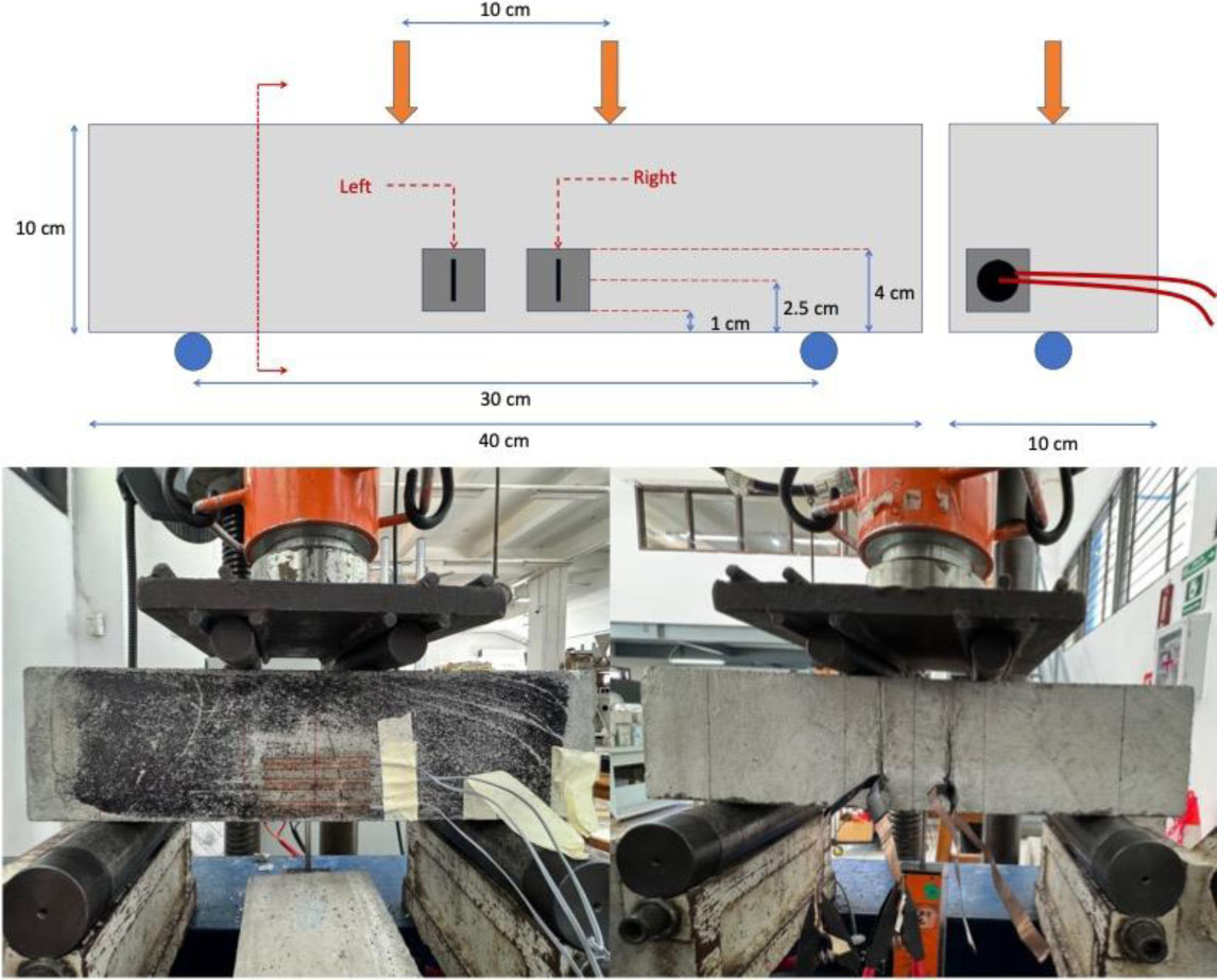
Figure 4:
Four-point bending test setup
3. Results and Discussion
3.1. Effective Frequency Range
The effective frequency range shows the increasing conductance value with increasing frequency and a decrease in the conductance value with the mortar aging (Pan & Huang, 2020; Pan et al., 2019). The conductance values that coincide between days cannot be selected as the effective frequency range because it means that there is no decrease in conductance as the days increase. In this study, the flexural testing was conducted at 28 days of age. The effective frequency range was selected based on two observations: conductance increased with higher frequency and decreased with higher loads. This selection criterion aligns with findings from research conducted by Pan et al. (2019) (Pan et al., 2019). Knowing the effective frequency range is important for optimizing structural health monitoring with EMI-based methods. It can increase the sensitivity, accuracy, and efficiency of the damage detection, leading to more reliable and effective maintenance and management of cement-based piezoelectric composites. Sensors can detect micro-damage in more detail.
In structural health monitoring with EMI-based, the broader effective frequency range indicates that the sensor actively responds to a broader spectrum of mechanical vibration and electrical impedance change. In addition, the broader the effective frequency range, the more frequency data, so that the conductance RMSD value will be more stable and more reflective of a change in the structure. Figure 5 shows the comparison of the beam conductance recorded by the CPCs.
According to this study, the effective frequency range for the mortar cube with an embedded C1 sensor was 500–1000 kHz. In addition, the effective frequencies for the cubes with embedded C2, C3, and C4 sensors were identified as 390–1000 kHz, 420–1000 kHz, and 300–1000 kHz, respectively. In this study, because there are two sensors (left and right) on one beam, the selected effective frequency range is the result of overlapping the frequency ranges between the two. For example, on beam C1, the effective frequency ranges of the left and right sensors are 610–730 kHz and 550–650 kHz, respectively. Thus, the effective frequency range representing the beam becomes narrower, namely 610–650 kHz. Figure 5 shows the frequencies of the beams with embedded C1, C2, C3, and C4 are 610–650 kHz, 430–730 kHz, 660–720 kHz, and 510–770 kHz, respectively. This data shows that the effective frequency range decreased as the dimension of the host structure increased.
Two sensors (left and right) were embedded within the flexural area of the beam. In the effective frequency range, conductance decreased as the applied load increased (This can be seen more clearly in the red box marked on each sensor in Figure 5). A comparison of the conductance recordings from the two sensors (left and right) is necessary to assess the consistency of performance in recording changes in beam conductance due to loading. At the effective frequency range, the average difference in conductance recorded between the left and right sensors of beam C1 reached 85%. Meanwhile, the percentage difference for beams C2 and C3 was 21% and 40%, respectively. The smallest percentage difference was shown by beam C4, which was only about 8%. Table 3 shows the effective frequency range of each beam along with the percentage difference in conductance recorded by the left and right sensors. The percentage difference in conductance is also shown in Figure 6.
Table 3:
The effective frequency range
| Variation | Effective Frequency Range [kHz] | Average Difference [%] |
|---|---|---|
| C1 | 610–650 | 85 |
| C2 | 430–730 | 21 |
| C3 | 660–720 | 40 |
| C4 | 510–770 | 8 |
C4 shows the smallest difference, while C1 shows the largest difference. This result indicates that polarization conditions (electric field and duration) affect how well CPC transduces and receives structural changes, as shown in the form of differences in conductance response to load changes and differences in left right sensor consistency. Higher electric fields and longer durations produce better polarization conditions, as indicated by the higher d33 value C4 (4.87 pC/N) compared to other variations (C3 = 4.67 pC/N, C2 = 4.60 pC/N, C1 = 4.63 pC/N) (Hayu et al., 2024). Sensors with better polarization conditions can detect mechanical energy more strongly, which is also demonstrated by a cleaner EMI conductance curve with less noise (higher SNR/Signal to Noise Ratio), shown in Figure 5. With a higher SNR, both conductance recorded on the beam tends to be closer.
Meanwhile, sensors with low polarization conditions, such as C1, have low sensitivity. This makes the sensor signal more affected by small differences in the interface area of each sensor with the mortar, such as microcracks, tiny voids, or embedment depth. These small irregularities become very apparent in the EMI results, which explains the large difference in conductance between the left and right sensors.
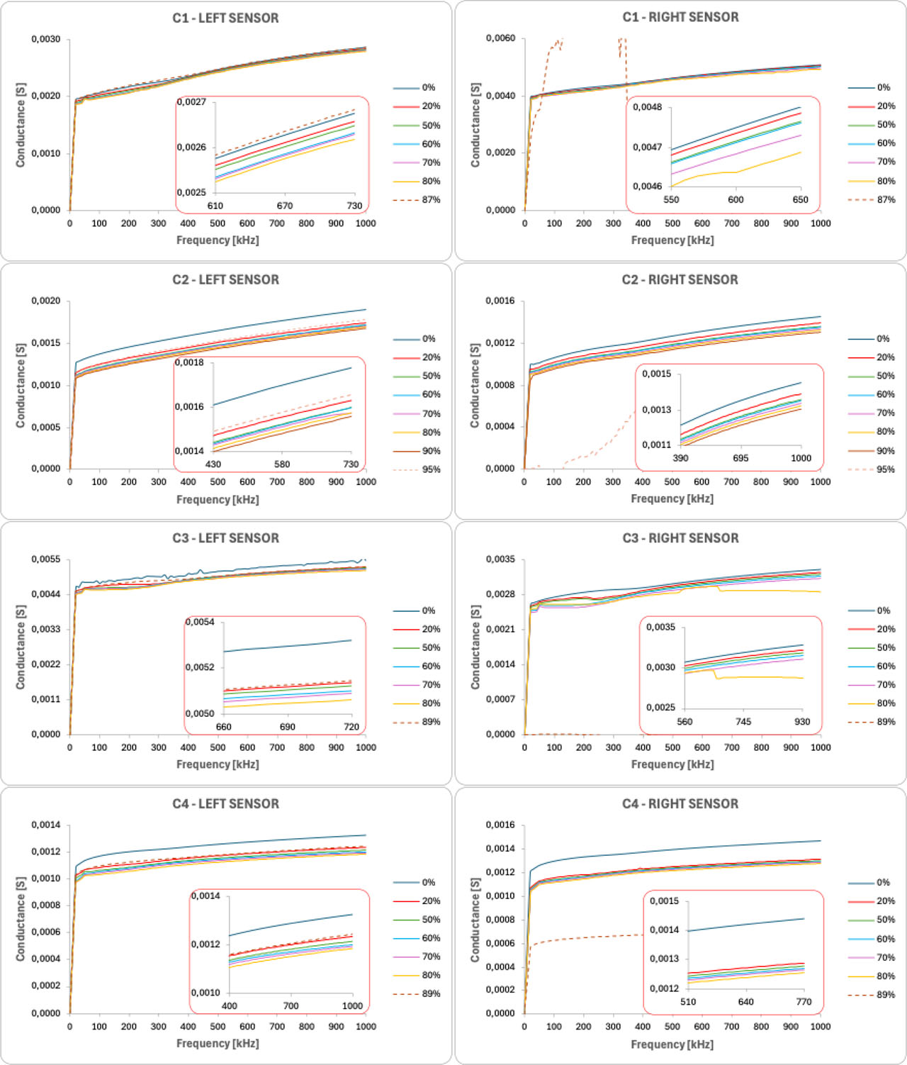
Figure 5:
Comparison of conductance response recorded from all tested beams
3.2. Conductance of Beam
The beam conductance recorded by the CPCs decreased as the applied load increased. The conductance values for beams C1, C2, C3, and C4 were higher than those for the corresponding cubes. In the effective frequency range, the C1 beam demonstrated a conductance range of 2.525×10⁻³–4.802×10⁻³ S, which was greater than the conductance of the C1 cubes, which ranged from 5.160×10⁻⁵–3.150×10⁻⁴ S. The ultimate bending load for the C1 beam reached 1162.51 kg, representing 87% of the maximum load capacity. During testing, crushing occurred at the right sensor, resulting in random fluctuations and a drop in conductance for that sensor, while the left sensor's conductance showed a slight increase.
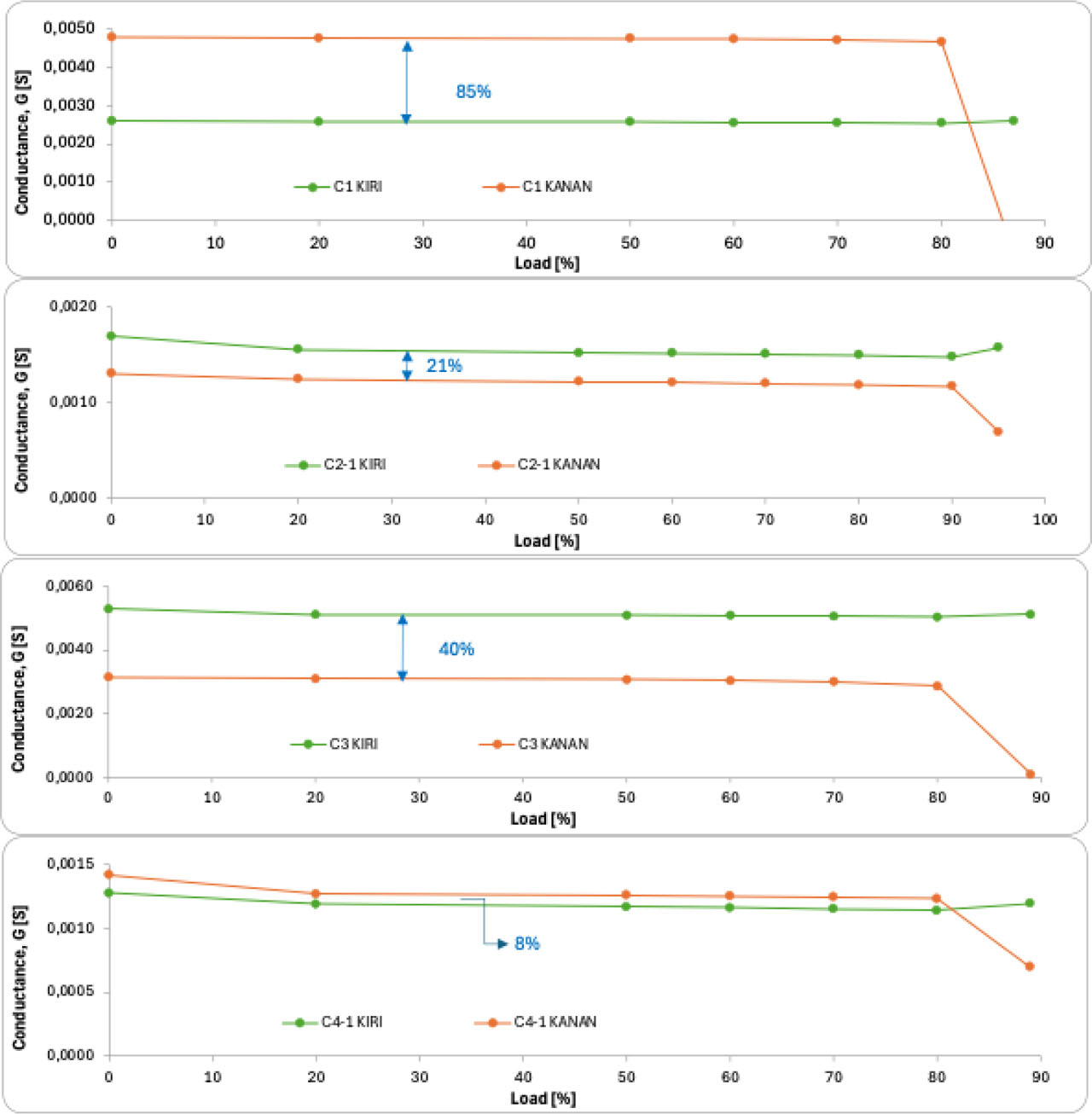
Figure 6:
Percentage difference in conductance between left and right sensors within the effective frequency range
Similarly, the C2 beam exhibited a conductance range of 1.108×10⁻³–1.777×10⁻² S, which was higher than the conductance of C2 cubes, recorded between 4.237 ×10⁻⁵–3.431×10⁻⁴ S. The crushing load for the C2 beam was 1262.45 kg, or 95% of the maximum load. The damage occurred at the right sensor, where its conductance also became random and dropped, while the conductance of the left sensor increased, mirroring the behavior observed in beam C1.
For the C3 beam, the conductance values ranged from 2.884×10⁻⁴ to 5.320×10⁻³ S, which outperformed the conductance of C3 cubes (5.679×10⁻⁵ to 3.415×10⁻⁴ S). The crushing load for the C3 beam was 1185.84 kg, or 89% of the maximum load. Destruction was noted at the right sensor, where its conductance values became random and increased significantly, while the left sensor's conductance also saw a slight increase. Lastly, the conductance of the C4 beam ranged from 1.125×10⁻³ to 1.441×10⁻³ S, higher than that of C4 cubes, which ranged from 3.989−5 to 3.134×10⁻⁴ S. The crushing load for beam C4 was 1182.51 kg, accounting for 89% of the maximum load. An anomaly occurred during the destruction of the beam. The right sensor became damaged along with the beam, while the left sensor remained intact. The destroyed sensor displayed erratic conductance changes, either spiking upwards or downwards, while the intact sensor showed an increase in conductivity. These conditions are depicted in Figure 6.
Table 4:
The standard deviation of conductance
| Variation | Load Stages [%] | Standard Deviation (S) | |
|---|---|---|---|
| Left Sensor | Right Sensor | ||
| C1 (610–650 kHz) | 0 | 3.407 ×10⁻⁷ | 3.975 ×10⁻⁷ |
| 20 | 5.973 ×10⁻⁷ | 1.988 ×10⁻⁷ | |
| 50 | 7.721 ×10⁻⁷ | 3.715 ×10⁻⁷ | |
| 60 | 6.341 ×10⁻⁷ | 4.184 ×10⁻⁷ | |
| 70 | 6.596 ×10⁻⁷ | 3.385 ×10⁻⁷ | |
| 80 | 6.434 ×10⁻⁷ | 6.133 ×10⁻¹⁹ | |
| C2 (430–730 kHz) | 0 | 4.419 ×10⁻⁶ | 4.338 ×10⁻⁶ |
| 20 | 2.469 ×10⁻⁶ | 2.876 ×10⁻⁶ | |
| 50 | 2.758 ×10⁻⁶ | 2.247 ×10⁻⁶ | |
| 60 | 3.900 ×10⁻⁶ | 2.134 ×10⁻⁶ | |
| 70 | 3.916 ×10⁻⁶ | 1.951 ×10⁻⁶ | |
| 80 | 3.102 ×10⁻⁶ | 1.840 ×10⁻⁶ | |
| 90 | 2.638 ×10⁻⁶ | 1.819 ×10⁻⁶ | |
| C3 (660–720 kHz) | 0 | 1.069E-06 | 2.005 ×10⁻⁷ |
| 20 | 2.742 ×10⁻⁷ | 1.004 ×10⁻⁶ | |
| 50 | 4.681 ×10⁻⁷ | 1.074 ×10⁻⁶ | |
| 60 | 1.048 ×10⁻⁶ | 4.357 ×10⁻⁷ | |
| 70 | 2.374 ×10⁻⁷ | 2.736 ×10⁻⁷ | |
| 80 | 3.286 ×10⁻⁷ | 2.757 ×10⁻⁶ | |
| C4 (510–770 kHz) | 0 | 3.787 ×10⁻⁶ | 2.926 ×10⁻⁶ |
| 20 | 2.858 ×10⁻⁶ | 2.847 ×10⁻⁶ | |
| 50 | 2.569 ×10⁻⁶ | 2.630 ×10⁻⁶ | |
| 60 | 1.825 ×10⁻⁶ | 2.572 ×10⁻⁶ | |
| 70 | 2.040 ×10⁻⁶ | 2.839 ×10⁻⁶ | |
| 80 | 2.622 ×10⁻⁶ | 2.667 ×10⁻⁶ | |
For conductance, the measurement uncertainty was evaluated from the residuals between the measured conductance response and its fitted curve. Calculations are performed for each loading stage and for each left and right sensor. The standard deviation (σ) was then extracted from these residuals. From Table 4, the results indicate that the relative standard deviation was very small compared to the absolute conductance values of each sensor. This is mainly because the uncertainty estimation was carried out only within the effective frequency bandwidth—the region where the electromechanical response is stable and usable. This highlights that selecting the effective frequency range is a critical step. It isolates the frequency window where the electromechanical coupling is dominant and avoids parasitic or irrelevant regions. By restricting the uncertainty calculation to this active frequency band, the estimated uncertainty becomes more representative of the true sensor behavior and more physically accurate.
3.3. Conductance RMSD
Beam conductance under each incremental load was quantified by comparing it to the baseline conductance, representing the initial state before any loading occurred. This quantitative method is known as Root-Mean Square Deviation (RMSD). The conductance RMSD was calculated within a selected effective frequency range. RMSD is a statistical measure used to evaluate the difference in conductance at loading levels of 20%, 50%, 60%, 70%, 80% and 90%, compared to the initial state with 0% load. In the CPC, RMSD helps assess conductance deviations over time or across different samples.
Conductance RMSD analyzed the crack's progression alongside beam strain, which was captured by a strain gauge. The C1 beam strain showed a pronounced increase at 50% loading, recording a value of 54.460 με. In the case of conductance RMSD, the response of the right sensor showed a pronounced increase at 50% loading, whereas the left sensor showed a significant increase at 60% with the respective values of 0.0075 and 0.0160. This differential measurement underscores the discrepancy between conductance RMSD and strain measurement integration.
The same issue was observed with the conductance RMSD condition of the C2 beam, where the most significant percentage increase occurred when the load was raised from 20% to 50%. The conductance RMSD values for the left sensor at 20% and 50% loading were 0.0844 and 0.1030, respectively. For the right sensor, the values were 0.0424 and 0.0648. The increases for the left and right sensors were 22% and 53%, respectively.
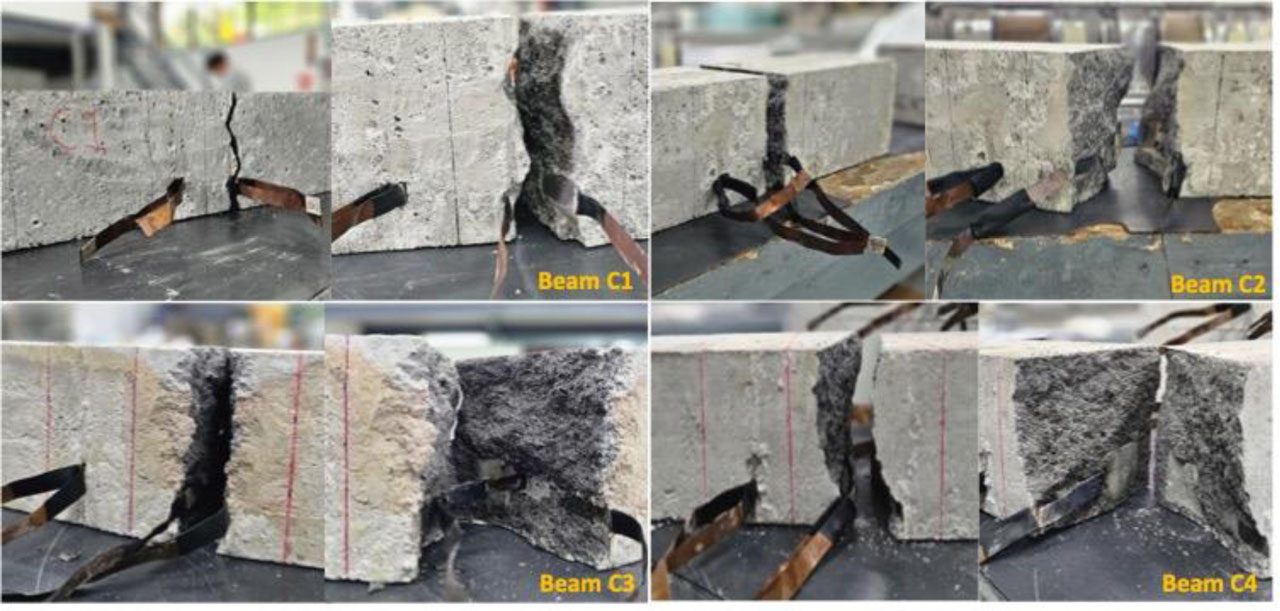
Figure 7:
Final damage condition of the tested beam after four-point bending failure
For the C3 beam, the strain at 50% loading increased dramatically to 47.887 με. The conductance RMSD increased significantly for the right sensor at 50% loading and the left sensor at 60% loading, which were 0.0248 and 0.0399, respectively. This indicates that strain values and conductance RMSD are not aligned. When the loading exceeded 80%, the conductance values exhibited increasing and decreasing spikes. The threshold for yield strain in mortar beams typically ranges from 80 to 400 με. The cracking strains of the C3 beam, which was 83.568 με, had already surpassed 80 με when the loading exceeded 80%. This is consistent with the experimental conditions, where the sensor and beam have been damaged when the load has exceeded 80%.
Table 5:
Range of conductance RMSD
| Variation | Range of Conductance RMSD [-] |
|---|---|
| C1 | 0,0032–0,0239 |
| C2 | 0,0424–0,1275 |
| C3 | 0,0149–0,0803 |
| C4 | 0,0675–0,1281 |
In the C4 beam, the most significant percentage increase occurred when the load was increased from 20% to 50%. The conductance RMSD of the left sensor at 20% and 50% loading are 0.0675 and 0.0822, while for the right sensor were 0.1046 and 0.1119. The percentage increase for the left and right sensors was 22% and 7%. Anomalies occurred when the loading exceeded 80%, and the recorded conductance values experienced spikes of increase and decrease. When the loading passed 80%, the strain had passed 80 με, so the beams had already cracked. This is in accordance with the experimental condition, where the sensors and beams collapsed when the load exceeded 80%. The trend reflects the alignment of the responsiveness of the C4 sensors to the loading.
Pan et al. (2019) conducted a similar study comparing PZT and CPC sensors embedded in concrete beams, with polarization at 1.5 kV/mm for 40 minutes (Pan et al., 2019). They found that conductance for the PZT sensor was 16–22 × 10−3 S, which decreased with increasing load as well, consistent with this study and previous study (Fan et al., 2018; Gayakwad & Thiyagarajan, 2022; Sikdar et al., 2022; Ye et al., 2020). In this case, conductance values were 12–22 × 10−3 S for the CPC sensor increased with increasing load. The significant difference between the conductance values in the Pan et al. (2019) study and this study is due to the higher polarization field applied, which increases the sensor's ability to generate an electrical signal. The RMSD of conductance for both the PZT and the CPC sensors increased similarly with increasing flexural load ranging approximately from 0.025–0.33 for PZT and 0.01–0.25 for CPC. This RMSD trend is consistent with the results in this study as well.
The RMSD uncertainty was quantified using the standard deviation (σ) of all RMSD values recorded under different load steps. For each CPC type, both left and right embedded sensors were included in the same data pool, because both sensors represent the same material configuration under the same loading sequence. Therefore, for each sensor type (C1, C2, C3, C4), all RMSD values from both sides were aggregated and treated as one statistical population. The standard deviation of this population was then calculated using the sample standard deviation method (n–1). This approach captures the natural variability of RMSD under incremental loading conditions, without requiring repeated mechanical tests, and reflects the intrinsic measurement dispersion of each CPC configuration.
Table 6:
The standard deviation of RMSD
| Variation | Standard Deviation [-] |
|---|---|
| C1 | 0,0105 ± 0,0079 |
| C2 | 0,0784 ± 0,0382 |
| C3 | 0,0340 ± 0,0224 |
| C4 | 0,1025 ± 0,0117 |
In the RMSD domain, the signal magnitude reflects the electromechanical sensitivity of the embedded sensor. A higher RMSD value indicates that the sensor produces a stronger electrical response per unit mechanical deformation; therefore, RMSD can be interpreted as an indicator of strain sensitivity. On the other hand, the standard deviation of RMSD across different load stages represents the stability of the sensor output, where a lower σ means lower fluctuation or noise in the RMSD signal. Sensor C4 showed the highest RMSD magnitude among all configurations, indicating that C4 is the most responsive against deformation progression. Importantly, C4 also exhibited the smallest standard deviation, which signifies that the RMSD signal produced by C4 is the most stable and repeatable. Therefore, C4 not only produced the strongest electromechanical response, but it also maintained the lowest signal variability. This combination clearly indicates that C4 provides the best balance between sensitivity (high RMSD) and measurement stability (low σ) and thus becomes the most reliable configuration in this study.
3.4. The Potential Use of CPCs in Beam
In EMI measurement, beams exhibit a narrower effective frequency range than cubes due to the physical and vibrational properties of the host structure. A larger structure has a greater mass and lower stiffness, resulting in a lower natural frequency. Consequently, the frequency peak occurs within a lower frequency (Guo et al., 2023; Hossain et al., 2015). A bigger structure has more internal micro damping. The amount of internal micro damping limits the effective frequency range. Consequently, the conductance spectrum tends to be flat at higher frequencies, causing a narrow effective frequency range. In a bigger structure, the wave propagation is longer. The longer wave propagation causes the reflected wave to be less intense due to dispersion and attenuation, resulting in fuzziness in the conductance detected at high frequencies. Unlike cubes, where the area is smaller, the wave can travel back and forth more strongly, allowing for a clearer recording of the increase in conductance. In a bigger structure, recorded conductance represents a small portion. This condition makes the EMI signal less sensitive at higher frequencies because it is less representative of the structure.
As the applied load increases, the stress level inside the mortar also increases, which initiates microcracks around and within the CPC sensor. The formation of these microcracks reduces the effective contact between the PZT particles and the cement matrix, thereby deteriorating the charge transfer pathways. Consequently, the electrical conduction performance of the composite becomes poorer as the damage progresses
In EMI techniques, conductivity refers to the extent to which electrical energy from the host structure is allowed to pass through the CPC sensors. From this study, the conductance value is greater than that of the corresponding cube. This is caused by:
A beam with a larger size can induce more electricity, resulting in increased conductance. This is because the beam has more volume to deform and vibrate.
With the same material, the stiffness of the beam is lower than that of the cube, so its mechanical vibration response is greater, which causes the sensor to record a higher amount of conductance. Meanwhile, the stiffness and compactness of the cube are higher, resulting in low mechanical energy transfer, which in turn leads to a lower electrical signal response (conductance).
Flexural loads have more dynamic deformations. Flexural loads create tensile and compressive zones in the beam simultaneously, resulting in a larger deformation gradient. Thus, the mechanical vibration response becomes larger, resulting in higher conductance. When compared to a cube subjected to a compressive load, the deformation that occurs is less dynamic bulk deformation. Since the cube is stiffer, the mechanical energy transfer is reduced, resulting in low conductance.
Among the four variations, the frequency range of C4 is the broadest compared to the other variations. In addition, the difference in conductance of the C4 beam in the effective frequency range between the left and right sensors is relatively small, at 8%. This percentage is the smallest value among the four variations. Among the four CPC variations, C4 shows the highest range of conductance RMSD. A high RMSD indicates a more significant difference between the baseline conductance and the conductance under incremental load. This indicates that C4 is more sensitive in recording conductance changes during mortar ageing. Conductance changes indicate microstructural changes in the mortar. Thus, C4 is the variant that best represents the development of mortar compressive strength.
4. Conclusion
The conclusion can be drawn from this study:
The results showed that the structural dimension plays a significant role in the electromechanical response of CPC sensors. The embedded sensors in the beam exhibited a noticeably narrower effective frequency bandwidth and higher conductance values when compared with those in smaller specimens (cubes), even under the same material composition.
Within the effective frequency band, all four CPC variants exhibited a consistent conductance response pattern: (i) conductance decreased with increasing bending load; and (ii) for a given load, conductance increased with increasing frequency within the effective band. At the onset of major damage (cracking), this pattern was disrupted, and conductance showed irregular fluctuations.
The measurement uncertainty estimated from the standard deviation of conductance within the effective frequency bandwidth at each loading step (and for both sensor sides) was found to be very small relative to the absolute conductance values. This highlights two important points: (i) defining the effective frequency bandwidth is a critical processing step because it isolates the most stable and physically meaningful electromechanical response; and (ii) the very small standard deviation confirms that the conductance response obtained from the embedded CPC sensors is highly reliable.
The conductance-based RMSD increased with increasing bending load, and the magnitude of the RMSD represents the electromechanical sensitivity of the embedded sensor. A higher RMSD value indicates a stronger electrical response per unit mechanical deformation.
Among all sensors, C4 showed the most stable performance with the smallest conductance difference between left and right sensors (8%) and the highest RMSD values (0.0675–0.1281). Importantly, C4 also exhibited the smallest RMSD standard deviation (0.1025 ± 0.0117), indicating that its RMSD signal was the most stable and repeatable. These results confirm that C4 provides the highest sensitivity in detecting microstructural changes.
Overall, these findings demonstrate that CPCs polarized under low electric fields are capable of functioning as effective embedded sensors for tracking microstructural changes induced by mechanical loading in larger structural elements (in this case, beams).
Acknowledgements
The authors also would like to acknowledge the vote of thanks to the Indonesian Endowment Fund for Education / Lembaga Pengelola Dana Pendidikan (LPDP) from the Ministry of Finance; Ministry of Research, Technology and Higher Education Indonesia; and Sepuluh Nopember Institute of Technology (ITS) for the financial support.
Notes
[1] Author Contributions
G.H. conceived the study, designed and performed the experiments, analysed data, and prepared the manuscript. W.S. supervised the research, contributed to data analysis-interpretation and reviewed the manuscript. K.W. provided technical support and assisted in experimental validation. P.S. supervised the research, reviewed the manuscript, and provided critical revisions and overall guidance. All authors critically reviewed and approved the final version of the manuscript and agreed to be accountable for all aspects of the work.