

1. Introduction
Soil salinization is one of the most significant factors in soil degradation (Prăvălie, 2021). It reduces water infiltration and storage capacity, leading to runoff and erosion (Shokri et al., 2024; Nofrizal et al., 2025). Soil salinization also reduces the activity of microorganisms and biodiversity (Haj-Amor et al., 2022). These problems are exacerbated by global climate change, as rising temperatures are accompanied by increased evaporation and decreased rainfall, particularly in arid and semi-arid regions (Khosravichenar et al., 2023). Soil salinization is estimated to threaten approximately half of the world's fertile lands (Singh, 2022). It is the most significant issue causing land degradation in Iraq's alluvial plain (Taleb Kadhum & Hussain, 2011; Hasab et al., 2015; Ziboon et al., 2022; Al-Jashaami et al., 2024; Jasim et al., 2024).
Laboratory-based salinity measurements provide highly accurate results; however, these methods can be time-consuming and labor-intensive, particularly over large areas. In recent years, remote sensing for salinity estimation has proven to be more efficient in terms of saving time, effort, and cost (Al-Helaly et al., 2022). Various models have been implemented, including linear, nonlinear, and machine-learning approaches. For example, Yu et al. employed the partial least squares regression (PLSR) method to estimate salinity in the western Song Plain of China, utilizing data from field surveys and Landsat 8 (Yu et al., 2023). Similarly, Alqasemi et al. utilized various remote sensing data along with in situ and laboratory measurements to detect salinity levels in Abu Dhabi, where they conducted regression analyses between the remote sensing data and the in situ and laboratory measurements (Alqasemi et al., 2021). El-Hamid et al. utilized a linear regression model to explore the relationship between remote sensing data, specifically data from the Operational Land Imager 8 (OLI) on Landsat, and ground laboratory samples. They then generated a spatial distribution of soil salinity using the Inverse Distance Weighting (IDW) method (El-Hamid et al., 2023). Several studies have utilized spatial interpolation through the IDW method to estimate the spatial distribution of salinized soils in various regions of Iraq. These studies relied on data from historical soil maps (Al-Arazah et al., 2021) or laboratory samples (Abdulhussein & Mihalache, 2022; Hammad et al., 2025), supplemented by remote sensing data. Additionally, some studies applied regression models to explore the relationship between laboratory samples and remote sensing data in the middle of the Iraqi alluvial plain (Al-Khuzaie et al., 2022; Abbas, 2023). On the other hand, some researchers applied the image classification method to investigate soil salinization. For example, Hassan and Hassan employed the Maximum Likelihood Algorithm (MLA) to classify satellite images, conducting their analysis based on results that did not include a calibration model linking laboratory samples to satellite images (Hassan & Hassan, 2024). Notably, none of the previous research considered the temporal dynamics of changes in soil salinization.
Machine learning algorithms have been widely applied in research related to estimating soil salinization using remote sensing data due to their effectiveness in handling nonlinear and non-stationary data. Poppiel et al. combined extensive laboratory data with Landsat 8 imagery in a study in midwestern Brazil, demonstrating that the Random Forest(RF) model is both robust and superior to other techniques (Poppiel et al., 2019). Similarly, Wang et al. employed various methodologies to predict salinity in southern Xianggan, China, concluding that the RF model produced the best results for estimating salinity from satellite images (Wang et al., 2020). Among machine learning models, the Extreme Gradient Boosting (XGBoost) model is also recognized as a reliable and accurate option for classification and regression tasks. In a study conducted by Maa et al., soil salinity maps were produced for the Ogan-Kuka River Oasis, located in the central and northern Tarim Basin of Xinjiang, China (Ma et al., 2021a). The researchers concluded that the XGBoost model outperformed both the Classification and Regression Tree (CART) and RF models. In another study by Zarei et al., which compared various machine learning models, it was found that XGBoost outperformed the Gradient Boosting Machine (GBM) and RF (Zarei et al., 2021). Mukhamediev and his team also concluded that XGBoost performed better in estimating salinity in the southern Kazakhstan study area compared to other models, including LightGBM, RF, Support Vector Machine(SVM), and Elastic Net (Mukhamediev et al., 2023). Additionally, a study conducted by Aksoy et al. focused on estimating soil salinity in Lake Urmia using Landsat 8 satellite data and ground observations (Aksoy et al., 2024). They employed two models, RF and XGBoost, concluding that XGBoost outperformed the RF model.
Estimates of soil salinity obtained from remote sensing are not solely dependent on the spatial and spectral resolution of satellite sensors (H. Chen et al., 2025). A well-designed data collection strategy plays a significant role in enhancing the accuracy of soil salinity estimates. Since soil is a continuous medium that exhibits considerable spatial and temporal variability, it is essential to adopt a methodology that incorporates time series data for soil salinization estimates.
In previous studies, researchers did not apply a specific data collection strategy based on time series. Our research aims to integrate two XGBoost models and feed them datasets from remote sensing, ground observations, and laboratory samples collected according to a specific strategy over two seasons: the wet season and the dry season, over a 12-year time series of data. The first model, Model A, is designed to identify soils containing vegetation residues (VR) or nonphotosynthetic vegetation (NPV) during the dry season. The second model, Model B, generates a final map that depicts the binary distribution of arable and non-arable soil based on soil salinity levels. Model A serves as an extraction mask for Model B, ensuring accurate classification.
2. Study area
Our research focuses on the Dhi Qar region of Iraq. Dhi Qar is located between latitudes 30° and 32° North and longitudes 45° and 47° East, encompassing a total area of 12,900 km2 (See Figure 1). The land cover and land use (LCLU) in this region feature a variety of environments, including agricultural lands, marshes, wetlands, grasslands, and barren areas (Zanaga et al., 2021). Specifically, the agricultural lands in Dhi Qar cover approximately 700 km2 (Tawfiq, 2020). A significant challenge facing Dhi Qar is soil salinization, a major contributor to soil degradation in the area (Hassan & Hassan, 2024; (Makki et al., 2025). This issue of salinization is worsening over time. The water sources in Dhi Qar include the Euphrates River, which flows into the southwestern part of the region, and the Gharraf River, which enters from the north and flows southward. It is important to note that the Gharraf River is a branch of the Tigris River.
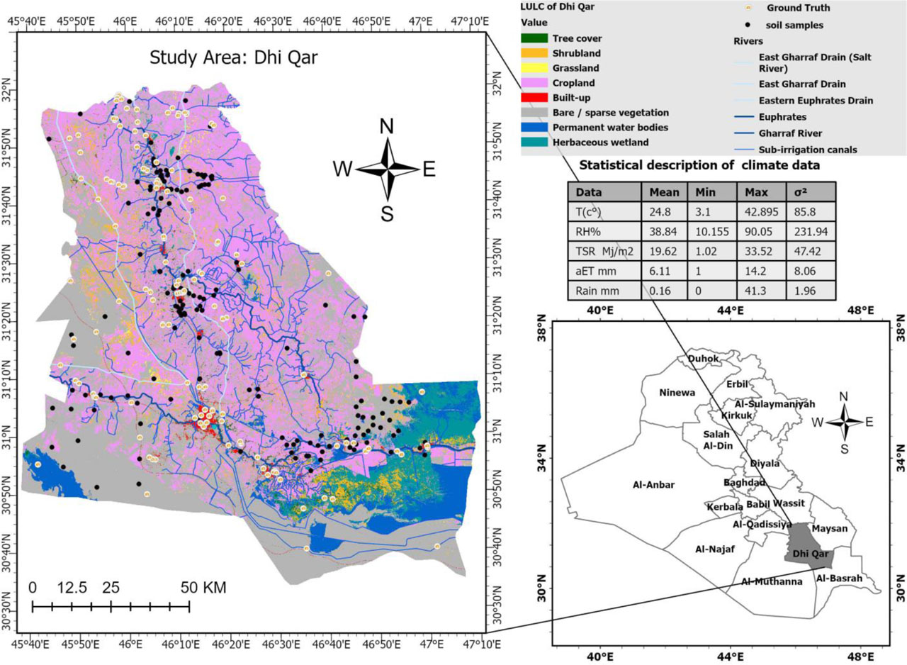
Figure 1:
Study area
The climate description of the study area is as follows: the mean rainfall was 0.16 mm, temperature (T) was 25°C, total solar radiation (TSL) was 20 MJ m−2, relative humidity (RH) was 39%, and aET was 6 mm. The maximum recorded values for these data were about 41 mm for rainfall, 43°C for T, 33 MJ m−2 for TSR, 90% for RH, and 14 mm for aET. Conversely, the minimum values measured were approximately 0 mm for rainfall, 3°C for T, 1 MJ m−2 for TSR, 10% for RH, and 1 mm for aET. This data is available on the Iraqi Ministry of Agriculture's meteorological website (https://www.agromet.gov.iq).
3. Materials and Methodology
Our research methodology involves several key steps. We start by collecting and processing remote sensing data, gathering ground truth data, and taking laboratory samples. This information is then compiled into a geodatabase, which is modeled and visualized using binary maps. See Figure 2.
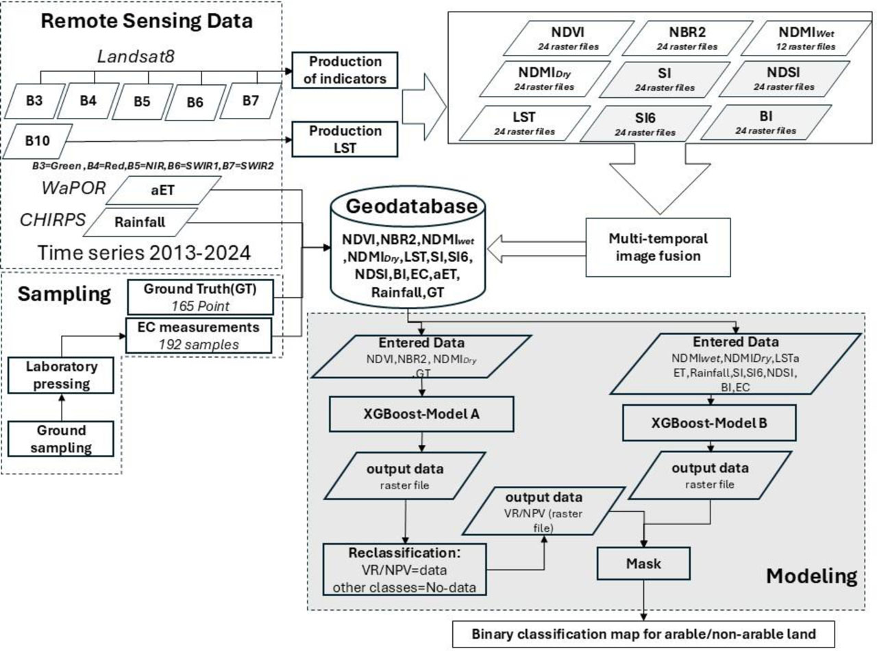
Figure 2:
Methodological framework for the research
4. Data collection
4.1. Remote Sensing Data
A total of 540 scenes from Landsat 8 were collected over 12 years, utilizing five different bands across three time periods. The first period corresponded to the wet season in March, while the other two occurred during the dry season in May and October. The bands included green (0.53–0.59 µm), red (0.64–0.67 µm), near-infrared (NIR) (0.85–0.88 µm), short-wave infrared 1 (SWIR1) (1.57–1.65 µm), and short-wave infrared 2 (SWIR2) (2.11–2.29 µm). Landsat 8 covers the Dhi Qar study area from three different paths and rows: path 166, row 39; path 167, row 38; and path 166, row 38. All scenes are from the Collection 2 Level-2 compilation, processed by the Earth Resources Observation and Science (EROS) Center. They have undergone radiometric and geometric corrections and possess a spatial resolution of 30 meters.
AET data were from the World Association for Public Opinion Research (WaPORv2 and v3), and rainfall data from the Rainfall Estimates from Rain Gauge and Satellite Observations (CHIRPS). Rainfall data was collected over a specific time window of four months, from the end of October/beginning of November to the beginning of March (wet season). See the Table for more details. This data collection approach leads to more accurate estimates of salinity, as saline soils typically demonstrate poor drainage.
Table 1:
The indicators and data used in the research
| Data/Index | Mathematical Formula | Source | Time |
|---|---|---|---|
| aET [mm] | ***************************** | WaPOR(v2and v3) | 2013–2024 |
| Rainfall [mm] | ***************************** | CHIRPS | 2013–2024 |
| NDVI [-] | Landsat8(B5,B4) | 2013–2024 | |
| NBR2 [-] | Landsat8(B6,B7) | 2013–2024 | |
| NDMI [-] | Landsat8(B5,B6) | 2013–2024 | |
| LST [kelvin] | ***************************** | Landsat8(B10) | 2013–2024 |
| SI [-] | Landsat8(B4,B3) | 2013–2024 | |
| SI6 [-] | Landsat8(B4,B5,B3) | 2013–2024 | |
| NDSI [-] | Landsat8(B4,B5) | 2013–2024 | |
| BI [-] | Landsat8(B3,B4,B5) | 2013–2024 | |
| River data [-] | ***************************** | NCWRM | 2013–2024 |
4.2. Field and Laboratory Data
In addition to the data obtained from Landsat 8, WaPOR and CHIRPS, 192 soil samples were collected and analyzed in the laboratory. Of these, 41 were analyzed by the authors, while the remaining data were sourced from previous studies (Ibrahim Hamad, 2016; Talib mujyfi, 2020; Al-Hamdawi & Al-Wally, 2020; Mohammed Haran, 2019; Hussein Al-Dubayani & Razzaq Al-Atabi, 2019) and National Center for Water Resources Management (NCWRM) (See Supplementary Materials Table S1). Laboratory data were collected over a period of time spanning from 2013 to 2024, which is helpful in monitoring dynamic changes in soil salinization.
The samples analyzed by the authors were collected at a depth of 30 cm and air-dried before being screened through a 2 mm sieve. Specific laboratory procedures were followed to determine the soil salt concentration, which refers to total soluble salts. The soil samples were mixed with distilled water and agitated to ensure complete dissolution. The electrical conductivity (EC) of the resulting soil solution was measured using a conductivity meter (HI 2300, HANNA) with a soil-to-water dilution ratio of 1:5. In this phase, the electrical conductivity of the soil-water extract was quantified in decisiemens/meter (dS/m). The average EC reading from the 192 samples is 15.60 dS/m. The standard deviation is ±23.62 dS/m, and the variance is 558.32 dS/m. The maximum recorded value is 152.60 dS/m, while the minimum is 1.29 dS/m. Additionally, the skewness is 3.18, and the kurtosis is 12.26. See Figure 3. The statistical summary of EC(dS/m), read EC (s distinctly illustrates the significant variability in soil salinity within the study area.
A total of 164 ground truth points were recorded. The coordinates of these points were obtained using a Garmin GPS device. This coordinate system is compatible with both remote sensing data and laboratory soil samples, explicitly using the UTM/WGS-84 zone 38N. Seventy-two of these points were visited in the field, representing soil that contains VR and NPV. See Figure 4. The remaining points were collected from high-resolution satellite images from ESRI (Esri, 2025).
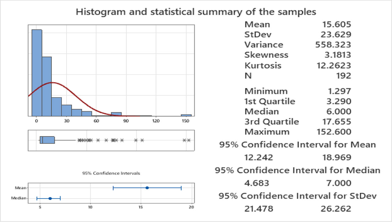
Figure 3:
Histogram and summary statistics for soil samples
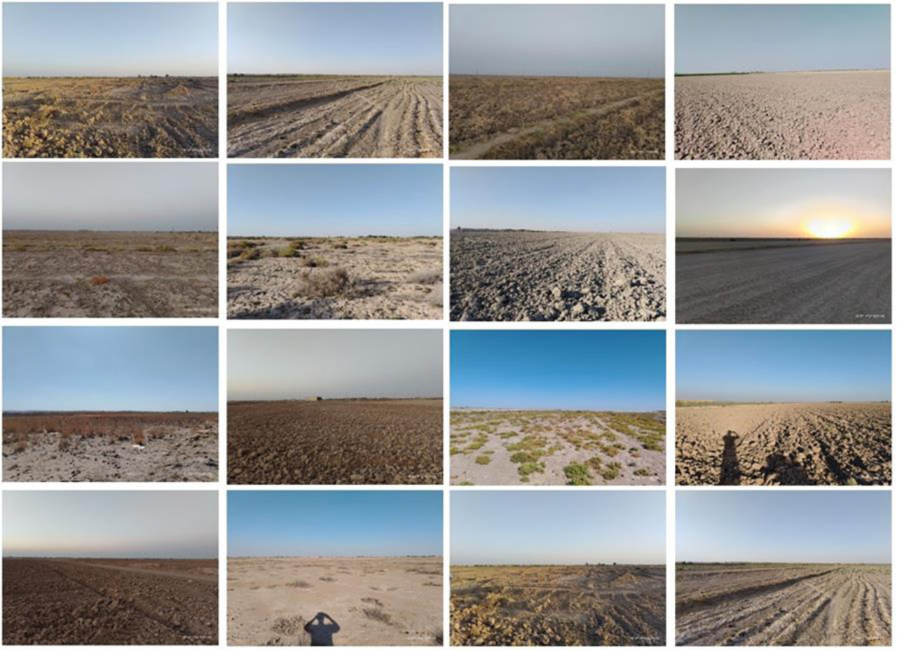
Figure 4:
Ground truth points
4.3. Data Preprocessing and Index Calculation
The 540 scenes from Landsat 8 were mosaicked and clipped to align with the study area, which resulted in a single raster file for each band. This process was carried out using ArcGIS Pro 3.4. We then used the generated raster files for each band to calculate the NDVI, NBR2, NDMI, LST, salinity index (SI), salinity index 6(SI6), Normalized Difference Salinity Index (NDSI), and Brightness Index (BI). Additionally, the cumulative annual rainfall and annual aET data were clipped and resampled to a 30-meter resolution.
The NDMI is calculated using bands B5 (NIR) and B6 (SWIR1), as detailed in Table 1. The moisture index is calculated during both the dry season (NDMIdry) and the wet season (NDMIwet). Analyzing the combined rainfall alongside the moisture index during the wet season enhances our understanding of how soil absorbs moisture from rainfall. During the dry season, aET and LST provide insights into the amount of water evaporating from the soil, which improves predictions of salinization.
The NDVI and NBR2 were calculated using the B5 (NIR), B4 (Red), B6 (SWIR1), and B7 (SWIR2) bands in the dry season, as indicated in the mathematical formula in Table 1. We utilize the NDVI, NBR2, and NDMIdry to generate a binary classification of soils containing vegetation residues (VR) or non-photosynthetic vegetation (NPV) in the dry season and other land cover/land use (LULC) categories, such as built-up areas, water bodies, and wetlands. The dry season corresponds to the non-planting season in agricultural regions. By combining NDVI, NBR2, and NDMIdry, we can differentiate between previously cultivated land, land with VR, NPV, and areas that remain barren throughout the year. The NBR2 is particularly effective at detecting VR and NPV, while the NDVI is excellent for identifying pixels that represent bare land (Demattê et al., 2018; de Sousa et al., 2024) and is also effective in detecting photosynthetic vegetation (Kadhim et al., 2022). On the other hand, using the vegetation index in conjunction with the moisture index provides a more accurate estimate of isolating land cover classes (such as water bodies and wetlands), and soil that contains VR, and NPV.
Four salinity indices—SI, SI6, NDSI, and BI—are applied because they have been widely used in previous research and effectively detect soil salinity (Gorji et al., 2020; Omuto et al., 2021; Jiang et al., 2022). The mathematical combination of these indicators integrates visible and thermal components, enhancing the accuracy of soil salinization detection through satellite images(Nurmemet et al., 2015; El-Hamid et al., 2023; S. Chen et al., 2022; Raheem & Hatem, 2019). In our case the relevant bands are B3(Green), B4(Red), and B5(NIR). See Table 1.
Multi-temporal image fusion provides valuable insights into properties that may change over time under specific conditions. This technique allows us to collect detailed information on vegetation cover, soil salinity, and bare soil from 2013 to 2024 in our study area. In our research, we employed a fusion method that calculates the mean of raster files generated from Landsat for various salinity indicators, including NDSI, SI, SI6, and BI, as well as NDVI, NBR2, NDMI(wet and dry), and LST. The result of this process is labelled (fusion) for all data, resulting in the following outputs: NDSIfuion, SIfuion, SI6fuion, BIfuion, NDVIfuion, NBR2fuion, NDMIWetfuion, NDMIDryfuion and LSTfuion. See Figure 5.
5. Machine Learning Modeling
5.1. The XGBoost Algorithm
The XGBoost model is a widely utilized and efficient open-source implementation of the gradient-boosted trees algorithm developed by Chen and Guestrin (T. Chen & Guestrin, 2016). The XGBoost operates significantly faster and requires considerably fewer computational resources and internal storage compared to traditional machine learning models. XGBoost model is a supervised learning algorithm designed to predict a target variable with precision by aggregating the predictions of multiple simpler and weaker models, a concept known as “boosting,” which enhances a “strong” learner from a collection of “weak” learners (Hakkal & Lahcen, 2024). In the XGBoost model for regression and classification, the weak learners consist of regression trees, each of which assigns an input data point to one of its leaves that contains a continuous score. The XGBoost model optimizes a regularized objective function that integrates a convex loss function, which reflects the disparity between predicted and actual outputs, along with a penalty term for model complexity, specifically the regression tree functions. The training occurs iteratively, incorporating new trees that forecast the residuals or errors of preceding trees, which are subsequently amalgamated with earlier trees to generate the final prediction. The model is termed gradient boosting due to its utilization of a gradient descent algorithm to minimize loss when incorporating new models. Our study utilizes the XGBoost model within the ArcGIS Pro version 3.4 environment to model the relationship between laboratory samples, ground truth data, and remote sensing data.
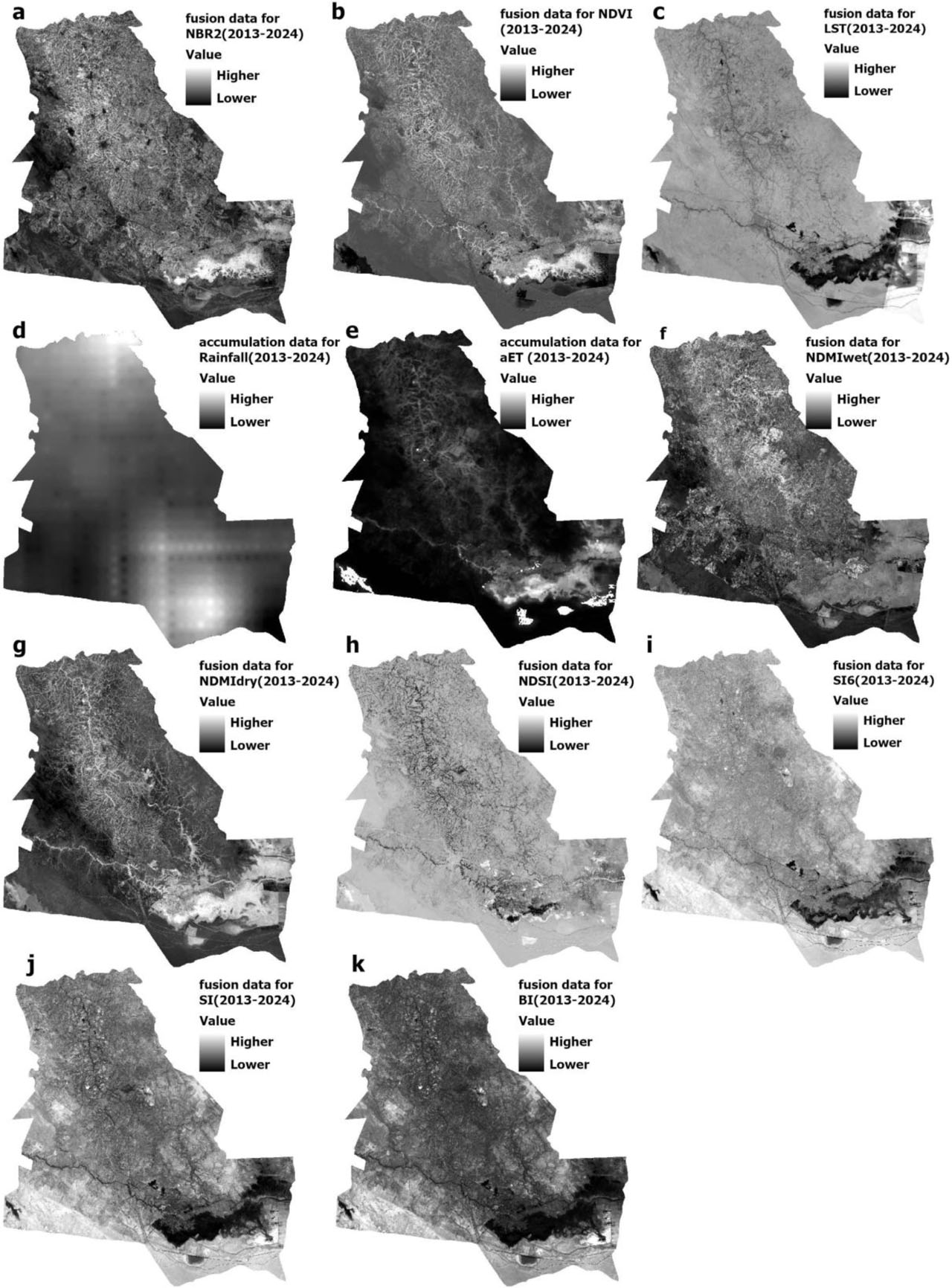
Figure 5:
Multi-temporal image fusion and cumulative data. a,b,c,f,g,h,I,j, and k multi-temporal image fusion for NBR2, NDVI, LST, NDMI (dry and wet season), NDSI, SI6, SI, and BI, respectively. d and e cumulative annual rainfall and aET data, respectively
5.2. Model A: Isolation of soil containing VR/NPV from other LULC categories
The VR/NPV-other class binary classification is a method used to differentiate soils that contain VR/NPV from other LULC categories. This approach utilizes the XGBoost model, resulting in a raster file that highlights areas of soil enriched with VR/NPV, indicating they are more fertile and suitable for agriculture. The “other” category in the binary classification encompasses either decertified soil, which is not arable throughout the year, or other categories of the LULC, such as water bodies. In our methodology, we assigned the label “Model A” to this model. See Figure 2. The Model A incorporates auxiliary data, including NDVIfuion, NBR2fuion, and NDMIDryfuion. Model A is calibrated using ground truth sampling. In our binary classification process, soil that contains plant debris is labeled as “SoilVR/NPV,” while all other LULC categories are classified as “other classes.” We utilized a total of 164 ground truth observations, which we divided into two groups: SoilVR/NPV and other classes. Ground truth observations for SoilVR/NPV were assigned a code of 1(presence), while observations not representing SoilVR/NPV were coded as 0 (absence). This classification is essential for preparing the data before it is input into XGBoost-Model A.
5.3. Model B: Binary classification of arable /non-arable soils
The binary classification of soil as arable or non-arable is based on the classification of EC(dS/m) readings, which indicate the soil's salinity level. Determining the EC(dS/m) threshold is essential for differentiating between soils with specific EC(dS/m) values and those that are suitable for cultivating various types of trees and crops. A soil with a higher EC(dS/m) value is conducive to the growth of particular plant species. We established a threshold of 7 dS/m for EC readings: soils with readings below this threshold are considered suitable for all crops (e.g., wheat), while readings above 7 dS/m are more suitable for halophytic plants, such as barley (Allan et al., 1998; Grieve et al., 2012).
The XGBoost model was utilized for the EC(dS/m)-based binary classification (Model B). See Figure 2. The EC values from laboratory-analyzed soil samples were used to calibrate the XGBoost-Model B. Readings below 7 dS/m are coded as 1 (present), and those above 7 dS/m are coded as 0 (absent). Additionally, the Model B incorporates auxiliary data, which includes four salinity indices (NDSIfuion, SIfuion, SI6fuion, BIfuion,), NDMIWetfuion, NDMIDryfuion, and LSTfuion, annual accumulation rainfall, annual accumulation aET, and river and irrigation channel data.
5.4. Hyperparameter Optimization for XGBoost
When using a machine learning model like XGBoost, there are no fixed criteria for determining its characteristics, such as the number of trees, leaf size, tree depth, and other parameters. These characteristics are flexible and can be adjusted to achieve optimal classification accuracy. To explore this further, we applied a parameter optimization method, specifically grid search. This optimization focused on maximizing the Matthews Correlation Coefficient (MCC) (See Equation 4 in the section Model Evaluation Method). During model optimization, we controlled the number of trees, leaf size, percentage of training data available per tree, and the range of tree depth. In addition to the MCC, we also monitored the model's performance using the F-score, accuracy, and sensitivity, which will be explained in the following paragraph. We applied model parameter optimization to both models, Model A and Model B.
5.5. Model Evaluation Method
To assess the model's performance in the binary classification, we utilized several metrics: accuracy (Equation 1), sensitivity (Equation 2), the F-score (Equation 3), and the MCC (Equation 4). The F1-score is a metric that combines accuracy and sensitivity, making it particularly suitable for addressing datasets with imbalanced categories. It provides a more comprehensive view of the model's overall performance. The MCC quantifies the effectiveness of binary classifications by considering all four components of a confusion matrix: true positives (TP), true negatives (TN), false positives (FP), and false negatives (FN). The MCC serves as a correlation coefficient that measures the relationship between predicted and actual classifications, with values ranging from −1 to +1. An MCC of +1 indicates perfect predictions, 0 signifies performance equivalent to random guessing, and −1 represents complete discord between predictions and actual results. Accuracy measures the number of correct predictions made by our model out of all predictions for a given category. In contrast, sensitivity measures the number of correct predictions out of all actual instances in the dataset for that category.
Where:
TP - True Positives,
TN - True Negatives,
FP - False Positives,
FN - False Negatives.
6. Result
6.1. Model A and Model B optimization parameters
The parameters for optimizing the XGBoost models (Model A and Model B) were set within the following constraints: the number of trees varied from 50 to 300, the leaf size ranged from 1 to 10, the tree depth ranged from 2 to 24, and the percentage of training data available per tree was between 40% and 100%. The learning rate (Eta) and L2 regularization (Lambda) were fixed at 0.3 and 1, respectively. In both models, 90% of the data was used for training, while the remaining 10% was reserved for validating the model's performance. For the Model A, the optimal parameters identified were 100 trees, a leaf size of 1, a tree depth ranging from 2 to 6, a mean tree depth of 3, 100% training data available per tree, and one random sample for the variables. In the case of the Model B, the best parameters found were 180 trees, a leaf size of 11, a tree depth ranging from 2 to 8, a mean tree depth of 3, 100% training data available per tree, and three random samples for the variables. See Table 2.
6.2. Predicting the spatial distribution of the SoilVR/NPV and other classes
Based on the optimization results for Model A, we used the model's hyperparameters to create a raster file that visualizes the binary classification of SoilVR/NPV versus other classes. The Model A achieved impressive performance in both the training and validation phases, with MCC values of 0.99 and 0.79, respectively. The F1-Scores were 0.99 in the training phase and 0.93 in the validation phase, while the accuracy rates were 0.99 in both the training and validation phases. See Table 3.
The sensitivity for the SoilVR/NPV was 1 in both the training and validation phases. For the other classes, sensitivity was 0.99 in the training phase and 0.78 in the validation phase. The results from Model A demonstrated excellent differentiation between SoilVR/NPV and other LULC classes. For instance, wetlands containing a mix of submerged vegetation and open water were accurately identified, along with urban areas, sandy soils, and archaeological sites that lack year-round vegetation cover (see figure 6a).
Table 2:
Modeles Characteristics
| Model Characteristics | XGBoost-Model A | XGBoost-Model B |
|---|---|---|
| Number of Trees [-] | 100 | 180 |
| Leaf Size [-] | 1 | 11 |
| Tree Depth Range [-] | 2–6 | 2–8 |
| Mean Tree Depth [-] | 3 | 3 |
| Percentage of Training Available per Tree [-] | 100 | 100 |
| Number of Randomly Sampled Variables [-] | 1 | 3 |
| Percentage of Training Data Excluded for Validation [-] | 10 | 10 |
| L2 Regularization (Lambda) [-] | 1.00 | 1.00 |
| Minimum Loss Reduction for Splits (Gamma) [-] | 0.00 | 0.00 |
| Learning Rate (Eta) [-] | 0.30 | 0.30 |
Table 3:
Model A performance
| Phases | F1-Score [-] | MCC [-] | Accuracy [-] | Category | Sensitivity [-] |
|---|---|---|---|---|---|
| Training | 0.99 | 0.99 | 0.99 | SoilVR/NPV | 1 |
| other classes | 0.99 | ||||
| Validation | 0.93 | 0.79 | 0.99 | SoilVR/NPV | 1 |
| other classes | 0.78 |
The next step involves reassigning pixel values from the binary classification output of Model A. This process is crucial for generating a raster file that identifies SoilVR/NPV. The resulting raster file will serve as a mask for the binary classification output of Model B. To achieve this, each pixel representing SoilVR/NPV will be assigned a value of 1, while the remaining pixels, which represent other classes, will be marked as “no data” (see Figure 6 b).
6.3. Predicting the spatial distribution of arable and non-arable lands
The Model B demonstrated outstanding performance during the training phase, achieving F-scores, MCC, and accuracy rates of 1. Furthermore, the sensitivity for both arable and non-arable soils was also 1 in this phase. These impressive results were attained using optimized hyperparameters for the XGBoost-Model B. In the validation phase, XGBoost-Model B performed satisfactorily, with an F-score of 0.94, an MCC of 0.90, and an accuracy of 0.95. The sensitivity for arable soils remained at 1, while the sensitivity for non-arable soils was 0.88. See Table 4.
Table 4:
Model B performance
| Phases | F1-Score [-] | MCC [-] | Accuracy [-] | Category | Sensitivity [-] |
|---|---|---|---|---|---|
| Training | 1 | 1 | 1 | arable | 1 |
| non-arable | 1 | ||||
| Validation | 0.94 | 0.90 | 0.95 | arable | 1 |
| non-arable | 0.88 |
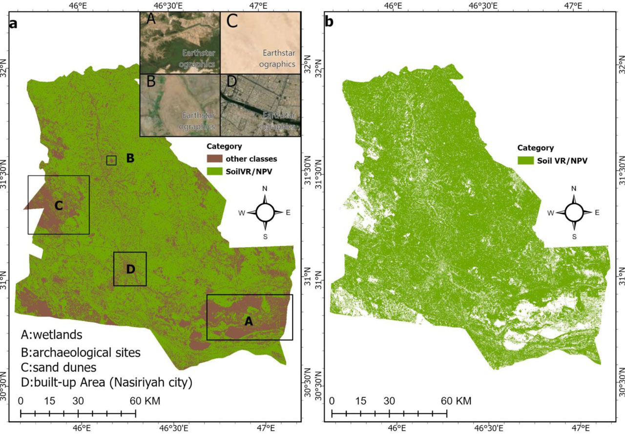
Figure 6:
Results of Model A. a -Binary classification of SoilVR/NPV and other LULC classes. b-Spatial distribution of SoilVR/NPV
6.4. Analysis of the Importance of Variables
The significance analysis of auxiliary data indicated that Rainfall, NDMIWetfuion, and LSTfuion were the most influential factors in Model B, with Gain values exceeding 10%. The NDMIDryfuion variable had a Gain of 9%, while the distance between rivers and samples contributed approximately 8%. Among the four salinity indices, NDSI and SI6 emerged as the most significant contributors to Model B, with Gains of 9% and 8%, respectively. See Figure 7. Rainfall and NDMIwet were the most significant contributing factors in Model B, together accounting for 14% of the total weight. Following closely was aET, which contributed approximately 12%, while LST accounted for around 11%, and NDMIdry contributed 8%. Among the salinity indices, SI6 was the strongest contributor to our model, accounting for approximately 12% of the overall weight.
6.5. Map of the Spatial distribution of arable and non-arable soil
The hyperparameters of Model B were used to predict the spatial distribution of arable and non-arable soil classes. A raster file generated from Model A, which represents SoilVR/NPV, served as an extraction mask to include only the pixels associated with SoilVR/NPV. This prediction process generated a binary raster file, where the first class represents arable land and the second class represents non-arable land, based on EC (dS/m). This binary raster file was then utilized to develop a spatial distribution map of arable and non-arable land (see Figure 8).
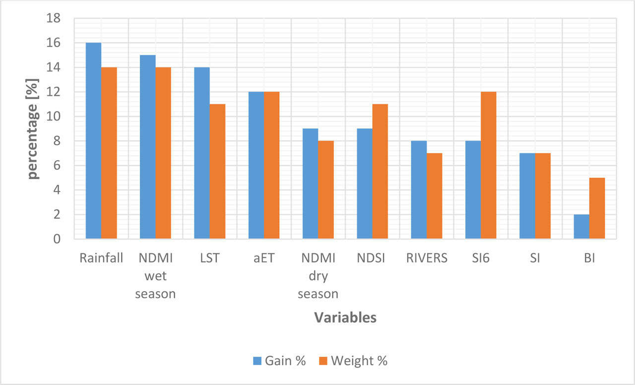
Figure 7:
Analysis of Gain and Weight Regarding the Importance of Variables
The results showed that there are 4,681 km2 of arable land with an EC value lower than 7 dS/m, which makes up approximately 58% of the total area. In contrast, non-arable land constitutes approximately 41% of the area, totaling 3,263 km2, with an EC value exceeding 7 dS/m. The spatial distribution of arable land is primarily concentrated in the center of the study area, particularly in the Gharraf River basin. A smaller portion of arable land is also found within the Euphrates River basin in the Dhi Qar study area.
7. Discussion
The results of this study are based on Landsat satellite data; although its performance is good, this may limit the results in this study. Furthermore, the laboratory data and ground truths used in calibrating the XGBoost model are specific to the study area, and this may be another limitation that should be taken into consideration.
The Model A demonstrated a high degree of accuracy in distinguishing SoilVR/NPV from other land cover classes (See Table 3). In this model, the auxiliary data included NDVI, NDMI, and NBR2, all derived from the visible and thermal bands of the Landsat 8 satellite over a specific time window. Using an index-based binary classification rather than a band-based classification proved to be more effective in differentiating specific classes, such as SoilVR/NPV, from other land cover types. This finding aligns with research by Brendel et al (Brendel et al., 2019) who indicated that employing index-based methods in conjunction with a robust classification approach yields improved results. Moreover, the inclusion of three indices in the XGBoost-Model A successfully distinguished SoilVR/NPV from other land cover classes, addressing a challenge researchers have faced in this field (Nguyen et al., 2021). Monitoring SoilVR/NPV is crucial for planning land use, informing agricultural practices, and developing policies that promote sustainable soil management. From Figure 6, we observe that most of the soil in this region contains VR or NPV, as there is little dense vegetation cover to shield the soil during the dry season. This lack of coverage exacerbates the salinization problem, as direct sunlight exposure increases the LST and aET leading to further degradation (de Sousa et al., 2024).
Analysis of the Importance of variables indicates that rainfall, humidity during the rainy season, and LST are the most influential factors affecting the performance of the Model B (see Figure 7). This observation suggests an increased likelihood of primary salinization in the study area, likely driven by rising temperatures and declining rainfall patterns associated with climate change (Tedeschi et al., 2023). This observation aligns with research by Wali et al. (Walli et al., 2025), which emphasized the significant impact of global climate change on soil salinization. Furthermore, poor water resource management, unsustainable irrigation practices, and excessive fertilizer application can worsen the situation, leading to secondary soil salinization. This observation is supported by Hassan and Hassan (Hassan & Hassan, 2024). A study by Muslim et al. (Muslim et al., 2023) confirmed that climate change, combined with inadequate land management due to intensive human activity, has intensified both primary and secondary soil salinization issues.
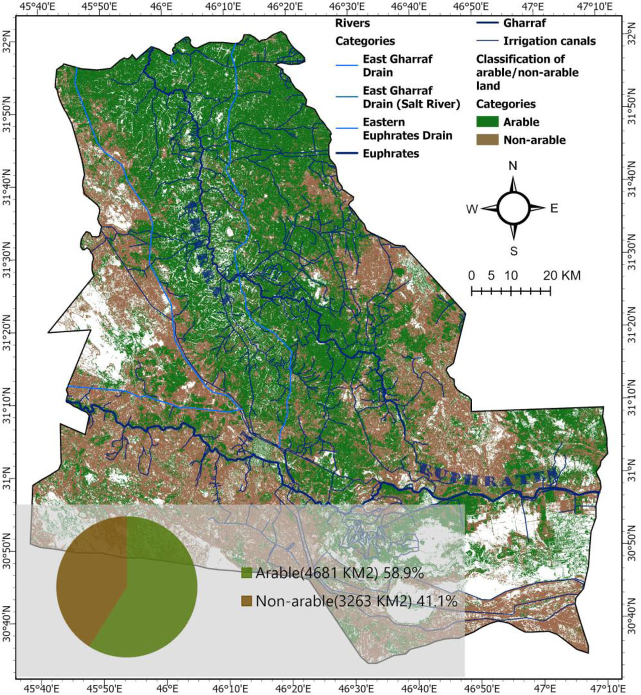
Figure 8:
Spatial distribution of arable/non-arable land
Furthermore, the most significant salinity index influencing the performance of Model B is the SI6. The mathematical component of SI6 integrates data from the visible spectrum (red and green) with near-infrared thermal data (see Table 1). As salinity accumulates in the soil due to decreased rainfall and increased evaporation, it can lead to the manifestation of salinity on the surface (Zheng et al., 2022), Which increases the soil's reflectivity of the electromagnetic spectrum within the visible and NIR range (Zhao et al., 2024; Kumar et al., 2024). This illustrates the effectiveness of SI6 in assessing salinity levels. Moreover, this supports the hypothesis that climate change significantly exacerbates the issue of soil salinization in the study area.
Utilizing remote sensing data to monitor soil salinization dynamics over an extended time series allows for effective and sustainable land management (Ma et al., 2021b; Hasan et al., 2021), ultimately reducing the costs associated with developing solutions to this issue. This is what we have reached in our study, where we have finally produced a map of the spatial distribution of arable and non-arable soils based on the amount of soil salinity. The spatial distribution map of arable and non-arable soils (Figure 8) illustrates that most of the arable land, characterized by an EC value of less than 7 dS/m, is located around the Gharraf River basin. In contrast, there is only a small amount of arable land near the Euphrates River basin. This difference can be attributed to the water quality of the two rivers. The Gharraf River, which originates from the Tigris River, is renowned for its high-quality water, making it suitable for irrigating a wide range of crops, as confirmed by Ewaid et al. (Ewaid et al., 2019). In comparison, the salinity levels of the Euphrates River are exceptionally high, as noted in a study by Hameed et al (Manar Majid Hameed et al., 2025).
8. Conclusions
Utilizing a time window across the time series of remote sensing data to estimate soil salinity, in conjunction with a robust classification model such as XGBoost, can produce accurate results. This methodology offers a time-efficient and cost-effective approach to monitoring the dynamics of soil salinization. By generating spatial maps of soil salinization, decision-makers gain a clearer understanding of optimal and sustainable land management practices. The methodology applied in our research can be implemented globally. Our secondary conclusions are as follows. Using an index-based binary classification instead of a band-based approach yields better results for specific land cover classes. Our results demonstrated excellent isolation of soils containing plant residues or non-photosynthetic vegetation during the dry season, indicating good soil quality. As a possible future direction, this method could be used to study the effects of intraseasonal drought and its impact on vegetation in any region around the world. From our findings, we observed that over half of the soils in the Dhi Qar study area have a salinity level of less than 7 dS/m. This spatial distribution is primarily located around the Gharraf River basin, suggesting that these soils are fertile.
Acknowledgements
The authors of this manuscript would like to express their gratitude to the National Center for Water Resources Management (NCWRM) for providing the necessary data, as well as to the Structural Laboratory at the Shatra Technical Institute for their assistance in conducting the required tests.
Notes
[1] Contributed by Author Contributions
Conceptualization, Mohammed H Azeez and Hisham M. Jawad Al Sharaa; data curation, Mohammed H Azeez; methodology, Mohammed H Azeez; software, Mohammed H Azeez; supervision, Hisham M. Jawad Al Sharaa, and Abdul Razzak T. Ziboon; validation, Mohammed H Azeez, Hisham M. Jawad Al Sharaa and Abdul Razzak T. Ziboon.; visualization, Mohammed H Azeez.; writing—original draft preparation, Mohammed H Azeez.; writing—review and editing, Hisham M. Jawad Al Sharaa, and Abdul Razzak T. Ziboon. All authors critically reviewed and approved the final version of the manuscript and agreed to be accountable for all aspects of the work.