
Positioning, navigation, and location monitoring have become indispensable elements of modern life, underlying a wide range of activities from transportation and logistics to socioeconomic planning and emergency response, including search and rescue operations. As these technologies are increasingly integrated into both daily routines and critical infrastructure, the demand for accurate and reliable positioning continues to grow.
Despite their widespread adoption, positioning systems remain vulnerable to various sources of errors. A common issue arises from discrepancies between the timing of the satellite system and the receiver’s internal clock, which can introduce inaccuracies. Furthermore, radio frequency interference can distort satellite signals during transmission, further affecting positioning performance. Among these challenges, multipath interference is one of the most persistent and problematic.
Multipath occurs when GNSS signals reflect off nearby surfaces, such as buildings, trees, bodies of water, or other large objects, before reaching the receiver. Instead of traveling directly from the satellite to the antenna, the signals arrive via multiple paths due to these reflections. The receiver then detects both direct and reflected signals, causing delays and signal distortion. These distortions primarily affect the timing and phase of the signal, which are critical for accurate position estimation. As a result, multipath can lead to significant positioning errors, sometimes reaching a few meters, depending on the environment and application (Peretic Matt (2025)).
To mitigate this issue, several strategies have been developed. One widely used solution involves the use of specialized GNSS antennas that are designed to suppress reflected signals. Additionally, advanced signal processing techniques and anti-interference algorithms have been implemented to identify and compensate for multipath effects. Although no method can entirely eliminate multipath interference, numerous studies have demonstrated that antenna-based solutions—such as right-hand circularly polarized (RHCP) antennas designed to preferentially receive the direct GNSS signal, and choke-ring antennas—and advanced signal processing techniques can significantly reduce multipath effects and improve GNSS positioning accuracy ((Teunissen et al, (2017)), (Chen et al., (2021)), (Xue et al., (2020)).
This study presents a novel data processing framework to mitigate persistent multipath interference in GNSS by integrating Differential GNSS (DGNSS) techniques with machine learning models such as Support Vector Machine (SVM), Convolutional Neural Network (CNN), and Random Forest. The methodology involves collecting synchronized GNSS data from a stationary base station and a mobile rover using high-precision u-blox ZED-F9P receivers with polarized antennas. After careful preprocessing and DGNSS correction—through single and double differences in pseudorange and carrier phase—feature vectors are constructed from both corrected and raw observation data. Labels indicating signal quality (“Clean” or “Noise”) are derived via skyplot analysis and building-induced obstruction modeling. Three classification strategies are explored: (1) direct use of DGNSS-derived vectors, (2) image-based classification, and (3) combined feature vector classification. Experimental results confirm that this integrated approach effectively identifies and excludes compromised satellite signals, thus improving positioning accuracy and robustness in challenging environments.
Multipath signals in GNSS systems are typically generated by reflections from surrounding objects, such as buildings, vehicles, and the ground, as well as by atmospheric propagation effects and, in some cases, reflections from the satellites themselves. These signals arise from the scattering of the direct line-of-sight (LOS) signal and possess distinct characteristics. In particular, multi-path signals travel longer paths than the LOS signal, resulting in delayed arrival times. Additionally, when reflections occur on passive, fixed surfaces, signal energy is inevitably attenuated as a result of reflection losses. The extended propagation distance further reduces signal power, making multipath signals generally weaker than their LOS counterparts. Given that GNSS signals, such as those from GPS L1, have wavelengths in the decimeter range, the delay introduced by multipath paths is often significantly larger than the carrier wavelength. As a result, the phase shift induced by multipath can be modeled as a uniformly distributed random variable throughout the interval [0,2π], especially in environments with rich scattering.
Detecting, mitigating, and eliminating multipath effects are essential to enhance the precision of satellite-based positioning systems. A widely adopted strategy involves the use of specially designed antennas that suppress the reception of signals affected by multiple paths. Among these, polarized antennas—particularly those employing right-hand circular polarization (RHCP)—are the most straightforward and effective solutions. GNSS signals transmitted directly via the line-of-sight (LOS) path are RHCP, whereas signals that undergo an odd number of reflections become left-hand circularly polarized (LHCP). Polarized antennas tuned to RHCP can therefore attenuate LHCP signals, effectively filtering out many multipath components. As a result, the received signal predominantly includes direct LOS signals and even-numbered reflected paths, which have less impact on positioning accuracy. This approach has been shown to significantly reduce positioning errors in multipath-rich urban environments, making it a practical and low-complexity solution for real-world GNSS applications (Chen J. (2021), Teunissen PJG (2017)). Its simplicity and robustness make polarized antennas especially suitable for urban deployments, where buildings and other structures frequently obstruct the GNSS signal path. However, the inherent limitation of this type of antenna is that it can only partially eliminate multipath signals, which can still lead to significant positioning errors. In GNSS, a more effective antenna design is the Choke Ring Antenna. The core idea of the Choke Ring Antenna is to use a shielding ring structure around the antenna to reduce the magnitude of multipath signals originating from low elevation angles, particularly those reflected from the ground. This design significantly decreases multipath signals by limiting reflections from sources below the horizon, thereby improving the quality of the received GNSS signals. The Choke Ring Antenna is an effective solution for suppressing multipath signals, which greatly contributes to the accuracy of GNSS systems. An inherent drawback of the Choke Ring Antenna is the reduced antenna gain at low elevation angles (below 20°). This reduction in gain means that the antenna will receive fewer satellite signals and weaker signal strength at these angles, leading to poorer GNSS signal quality and potential positioning errors (Xue Z. (2020)).
With the rise of smart cities, high-resolution 3D urban models have become increasingly accessible, driving advancements in GNSS positioning techniques that address multipath and NLOS errors. These methods, collectively known as 3D mapping-aided (3DMA) positioning, have gained significant attention. One of the most established 3DMA approaches is shadow matching (Groves P. D. (2011), Wang L. (2013)), which uses building outlines from 3D city models to determine satellite visibility. Other research efforts have focused on improving GNSS accuracy through the use of enhanced 3D digital maps (Betaille D. (2013), Peyraud S. (2013), Peyret F. (2014)). Moving beyond simply discarding NLOS signals, recent studies have investigated using NLOS signal paths constructively (Miura S. (2015), Peyret F. (2013)). These range-based 3DMA techniques combine ray-tracing simulations with hypothesis-driven positioning algorithms to estimate NLOS reflection paths and correct biased pseudorange measurements, achieving positioning accuracies within approximately meters in pedestrian environments (Hsu L.-T. (2016)). Nevertheless, the intensive computational requirements of ray-tracing and the limited real-time availability of detailed 3D building data pose challenges for implementation on low-cost GNSS receivers. Hsu L.-T. (2017) introduces a machine learning–based classifier aimed at distinguishing GNSS pseudorange measurements into three categories—clean, multipath, and non-line-of-sight (NLOS)—by leveraging features such as received signal strength and the consistency between pseudorange and Doppler shift measurements, achieving approximately 75% classification accuracy using a support vector machine (SVM) model.
Machine learning has been explored as an effective approach to enhance GNSS localization accuracy. Early research proposed a classification framework that evaluates positioning accuracy across three levels by incorporating factors such as satellite count, dilution of precision (DOP), received signal strength, and receiver velocity (Drawil N. M. (2013)). To detect biased pseudorange measurements, a Wilcoxon-norm regression model was applied to analyze the residuals of pseudorange data (Wang H.-S. (2013)). In static environments, elevation and azimuth angles were utilized as key input features in machine learning algorithms to mitigate the impact of multipath interference (Phan Q.-H. (2013)). Further advances included the use of signal processing variables derived from receiver internal correlators to classify six common GNSS receiver states (Sokhandan N. (2015)). Machine learning techniques for non-line-of-sight (NLOS) detection were incorporated into the Nav2Nav cooperative vehicle navigation system (Socharoentum M. (2016)), employing a decision tree classifier to distinguish line-of-sight (LOS) from NLOS signals based on received signal strength and elevation angle (Yozevitch R. (2016)).
In this study, we propose a framework for multipath detection and mitigation that includes key steps to address the challenge of detecting multipath interference in satellite positioning. The overview of the proposed framework is shown in Figure 1. The key steps include the following:
GNSS Data Collection: Raw GNSS data are collected simultaneously from a stationary Base station and a moving Rover. The Base provides correction messages in the RTCM3 format, while the Rover records raw measurements in the UBX format. This dual-format storage ensures compatibility with GNSS post-processing tools and supports accurate positioning through synchronized observation and correction data.
Data Pre-Processing: UBX and RTCM3 data are decoded and time synchronized to align Base station and Rover observations. Key measurements like pseudo-range, carrier phase, and correction messages are extracted and organized. This synchronized data set enables accurate DGNSS processing and supports further analysis such as feature extraction and signal quality assessment.
Data Processing using DGNSS: DGNSS processing is used to correct Rover measurements using Base station corrections, reducing errors like satellite clock and atmospheric delays. The result is a set of high-precision, time-stamped vectors of corrected pseudo-range and carrier phase data for all visible satellites at each epoch. These vectors form Data set 1, which supports later positioning and analysis tasks.
Extracting observation features combining with DGNSS data: Raw satellite observation features and DGNSS-corrected measurements are combined to form a unified feature vector for each satellite at every epoch. This includes features such as C/N0, Doppler, elevation, azimuth, corrected pseudo-range, and carrier phase. The resulting Data set 2 provides a detailed, time-stamped representation of each satellite’s signal characteristics, supporting advanced analysis and machine learning tasks.
Classification for multipath detection:
Approach 1 uses DGNSS-corrected measurement vectors from Data set 1 to classify signal quality as “Clean” or “Noise.” Machine learning models such as SVM, Decision Trees, and Random Forests are trained on these vectors to detect anomalies based on the structure of corrected pseudo-range and carrier-phase data. This method relies solely on refined DGNSS measurements for classification.
Approach 2 converts the sequences of the DGNSS-corrected measurements into visual representations, such as trend graphs or graphs, to capture temporal and structural patterns. Image-based features, such as HOG, are extracted from these visualizations and used to train classifiers like CNN or SVM to detect “clean” vs. “noise” conditions. This method combines time-series dynamics with spatial feature analysis for improved classification accuracy.
Approach 3 uses combined feature vectors from Data set 2 - containing observation metrics and DGNSS corrected - to classify signal integrity at the satellite level. Classifiers such as SVMs, Decision Trees and gradient-boosted trees are trained to distinguish “clean” from “noise” based on these rich feature sets. Feature importance analysis is also performed to identify which metrics are most relevant for detecting multipath or noise, providing valuable insights for diagnostics and model improvement.

The workflow of proposed methods for multipath detection
As mentioned in the previous section, to collect satellite data, the system employs a combination of a mobile receiver (Rover) and a fixed reference station (Base station). The Rover is specifically designed for field deployment, equipped with a high-precision u-blox ZED-F9P GNSS receiver and a specialized polarized antenna that effectively minimizes the impact of multipath interference. Figure 2 shows the pictures of polarized antenna and u-blox ZED-F9P GNSS receiver used in our experiments. This setup ensures reliable and accurate data collection in dynamic environments.

Polarized antenna and u-blox receiver module
As Differential GNSS (DGNSS) requires both a mobile and a stationary reference receiver, the Base station plays a critical role. It must be placed at a location with a precisely known position and minimal multipath interference. For this purpose, we use a Base station that is part of Vietnam’s official GNSS network, managed by the Ministry of Natural Resources and Environment. This choice ensures stable and accurate correction data for high-precision GNSS applications.
In our experiments, data are collected along the path between two buildings, as shown in Figure 3. Specifically, the u-blox positioning module was connected to the polarized antenna and a computer to collect satellite data in this area. During the data collection process using the u-center software, positioning accuracy metrics such as 3D accuracy, 2D accuracy, PDOP, and HDOP showed very high values. This indicates that the area between two buildings in our experiment is heavily affected by multipath interference.
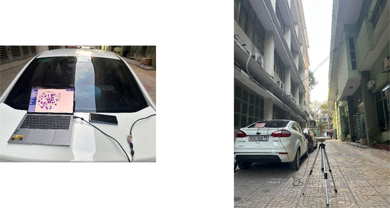
Data collection at an area between two buildings in our experiment
Once the rover receiver is in the field, satellite data collection begins using RTKNAVI, a component of the RTKLIB software suite (Version 2.2.1 is used in our experiment). RTKNAVI provides real-time monitoring and logging of GNSS data. The data acquisition process involves two primary data streams. The first is raw satellite signal data collected by the Rover receiver, which is transmitted to a computer through a serial interface. Within RTKNAVI, the appropriate communication parameters must be configured to ensure seamless data logging. These raw data are saved in the UBX format, a proprietary u-blox binary format designed for efficient storage of GNSS measurements. The second data source is the correction information from the Base station. RTKNAVI is set up to receive these corrections using the NTRIP (Networked Transport of RTCM via Internet Protocol). Through a network connection, the Rover accesses real-time RTK correction data broadcasted by the Base station. These correction data are saved in the standard RTCM3 format, which is widely used in GNSS for differential corrections.
These two data streams, Rover UBX files and Base station RTCM3 files, form the raw input for subsequent processing. In the following stage, the system decodes and standardizes these files to ensure consistent formatting and compatibility. This standardization step is essential as it prepares the data sets for the processing procedures used in subsequent phases, enabling accurate positioning and advanced GNSS analysis.
The collected satellite data are stored in two specialized file formats: UBX and RTCM3, each requiring a different processing method. For UBX files, which use a proprietary binary protocol developed by u-blox for their GNSS/GPS receiver modules, the program leverages the Python pyubx2 library to decode and extract relevant data.
As highlighted earlier, precise GNSS positioning depends on two key range measurements per satellite: pseudo-range and carrier phase. The program extracts these critical fields from the UBX file to support downstream positioning computations. In addition, it retrieves additional information, such as timestamp, satellite constellation, satellite ID, and signal type, all of which are valuable for in-depth analysis and quality assessment.
The main steps in processing UBX data are as follows:
Convert raw binary data into a readable string format for easier observation and extraction.
Extract key fields, including: Time (signal reception time), Satellite Group, Satellite Group Number (ID within the group), Pseudo-range (P1/C1), Carrier phase (L1)
Filter and retain only the primary satellite constellations of interest: GPS
For processing RTCM3 data (Radio Technical Commission for Maritime Services, Version 3 standard), the Python pyrtcm library is available. However, unlike UBX files, RTCM3 data does not directly provide essential GNSS measurements such as pseudo-range, carrier phase, or signal type. Extracting this information from RTCM3 messages is complex and time consuming and may not yield high accuracy. To overcome these limitations, RTCM3 data are first converted into OBS files (RINEX observation format) using RTKCONV, a tool from the RTKLIB software suite. RINEX (Receiver Independent Exchange Format) is a widely accepted and standardized format that simplifies GNSS data handling and ensures compatibility with various post-processing tools. This conversion ensures that the RTCM3 correction data are transformed into a standardized and accessible format, allowing efficient integration with the Rover observation data in later processing stages.
To simplify the program and improve the organization of the data, each RTCM3 file is split into four separate OBS files corresponding to the four main satellite systems: GPS, GLONASS, Galileo, and BeiDou, just as with the UBX data. The OBS file (RINEX observation format) contains the key fields required for GNSS data analysis, making it well suited for processing. It includes information such as the signal reception time (e.g., 24 4 26 9 51 13.000000, representing year, month, day, hour, minute, and second), the satellite constellation, and IDs (e.g., 8C 1C 2C 4C 5C 7C 8C 10C 13C, indicating 8 satellites with IDs C1, C2, C4), and essential measurements like pseudorange (C2) and carrier phase (L2). The program extracts these critical data fields and formats them to ensure compatibility between the Base station and Rover data sets. One key aspect of this process is time synchronization. The UBX file stores timestamps as the number of seconds since the most recent Sunday, whereas the OBS file uses absolute date and time. To align the two data sets, the program converts the OBS timestamps to the same time format used in the UBX files. This synchronization is vital for accurate differential processing in later stages, ensuring that measurements from both receivers correspond to the same epoch.
The final output of this satellite data processing step is the creation of two Excel data files: Base.xlsx and Rover.xlsx, each containing the same standardized data fields:
“Time” (synchronized time)
“Satellite-Number” (satellite ID)
“P1/C1” (pseudo-range)
“L1” (carrier phase)
After preprocessing the satellite data, the Rover and Base station datasets are merged based on two key fields: “Time” and “Satellite-Number”. Ensuring consistency in these fields across both datasets is essential for accurate alignment and meaningful analysis. The merged data set combines the corresponding measurements from Rover and Base for each satellite at each epoch, resulting in a unified data structure that includes the following fields.
“Time”
“Satellite-Number”
“P1/C1-r”: pseudo-range from Rover
“L1-r”: carrier phase from Rover
“P1/C1-b”: pseudo-range from Base
“L1-b”: carrier phase from Base
Once Rover and Base data sets have been successfully merged, the program applies the Differential GNSS (DGNSS) technique to improve positioning accuracy by removing common-mode errors. In DGNSS, it is assumed that the distances from a satellite to the Base station and to the Rover are significantly greater than the distance between the two receivers. This assumption allows us to consider the signal paths from the satellite to both receivers as nearly identical, meaning that many errors, such as ionospheric and tropospheric delays, are shared and can effectively be canceled.
To do this, the program first calculates the single difference of the pseudo-range measurements for each satellite i:
To further reduce these residual errors, the program computes the double difference by selecting another satellite k and calculating:
This double differencing removes remaining biases and isolates errors unique to specific satellite-receiver paths, especially those caused by multipath. Repeating this process across multiple satellite pairs, the program generates a time series of double-differenced values, which serve as input for subsequent processing steps.
This DGNSS method is applied to both pseudo-range and carrier phase data. For pseudo-range, the difference between Rover and Base for satellite i is computed as follows
Then, for each satellite, this value is subtracted from the differential measurements of all other satellites to compute the pseudo-range double difference, forming the foundation for advanced analysis such as noise detection and quality assessment.
The same differential approach used for pseudo-range measurements is also applied to the carrier phase. Specifically, the carrier phase difference between the Rover and the Base station for satellite i is calculated as follows
These computed deviations are subsequently organized into a time series that captures how errors between satellite pairs vary over time. Representing the data in this time series format provides several important advantages. First, it allows intuitive visualization and analysis of trend and error fluctuations, enabling the detection of patterns or anomalies that may not be evident in static data. More importantly, this time-series representation serves as a critical input for advanced algorithms aimed at detecting multipath interference. Multipath errors often exhibit characteristic temporal behaviors, and by modeling the evolution of error values over time, the algorithm can more effectively identify and isolate corrupted signals.
In summary, transforming differential measurements into a time series structure not only enhances interpretability and analytical depth but also plays a vital role in supporting accurate and robust multipath detection in subsequent processing stages.
For each satellite i, we construct a comprehensive feature vector that combines both features in the DGNSS-based and observation domain. First, we form satellite pairs by calculating the double differences in the pseudo-range and carrier phase measurements between the satellite i and every other satellite in view. From these pairwise differences, we compute statistical features such as the minimum, maximum, mean, and median for both pseudo-range and carrier phase values. These statistics capture the variation in the GNSS signal paths relative to other satellites, reflecting potential anomalies or irregularities in the satellite i’ signal.
In addition to the pairwise characteristics, we extract statistical summaries per satellite for satellite i based on its own observation data. These include the minimum, maximum, mean, and median values of parameters such as azimuth angle, elevation angle, Doppler shift, and carrier-to-noise ratio (C/N0).
The resulting feature vector for the satellite i thus encapsulates both the measurement discrepancies between the satellites and the geometric and signal quality characteristics specific to that satellite. This rich representation is well-suited for downstream tasks such as multipath detection, anomaly classification, or signal quality assessment.
To determine whether a satellite signal is affected by multipath or obstruction, environmental measurements are collected around the receiver. These include the height and horizontal distance of surrounding buildings. Using this information, the program assesses whether the satellite’s signal path is likely blocked based on its geometric position relative to these obstacles.
For each identified obstacle i, let α1,i, α2,i denote the azimuth bounds (in degrees) that define the angular sector blocked by the obstacle i. Let Ei represent the elevation threshold (in degrees). This threshold defines the minimum elevation angle that a satellite must have to be visible above the obstacle.
Let a satellite’s position be described by its azimuth angle and elevation angle. A satellite is considered blocked (i.e., potentially affected by multipath or non-line-of-sight propagation) if there exists any obstacle i such that:
If a satellite satisfies the condition in Equation (5) for at least one obstacle, it is labeled as Noise, indicating likely obstruction. Otherwise, it is considered to be in clear line of sight and is labeled as Clean.
The parameters α1,i, α2,i, Ei for each obstacle must be determined through on-site measurements or extracted from detailed terrain and building map data. These inputs are crucial for accurately modeling the satellite visibility environment and identifying signal degradation due to physical obstructions.
In our experiment setup, from the field layout diagram as shown in Figure 4, two main buildings are identified as potential signal blocking obstacles around the GNSS antenna:
Building 1: Bach Khoa Gymnasiums (northeast direction, 1.6 meters away, 9.0 meters high)
Building 2: TC Building (southwest direction, 2.4 meters away, 18.6 meters high)

Measuring the height and distance of the two buildings on two sides of the antenna
Using trigonometry, the elevation angles that these obstacles create (the minimum elevation a satellite must have to avoid being blocked) are calculated based on the height of the obstacle hi and the horizontal distance di to the obstacle building, according to Equation 6.
For Bach Khoa Gymnasiums buidling, the Azimuth range blocked: approximately 340° to 359° and 0° to 117°. For TC Building, the Azimuth range blocked: approximately 146° to 300°.
After measuring and computing the elevation thresholds and azimuth sectors, we summarize the blocked sectors as tuples of the form
These tuples can be used directly in the labeling logic: if the azimuth of a satellite lies between αmin and αmax (taking care of the wrap-around at 360 °) and its elevation is below Eth, then that satellite is considered obstructed (label “Noise”).
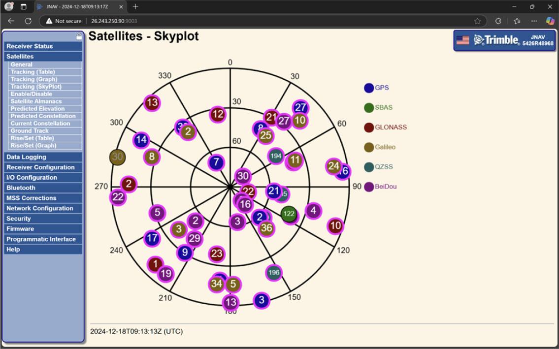
Skyplot indicated satellites’ azimuth and elevation
From the skyplot image, GPS satellites (indicated by blue circles) are identified along with their azimuth and elevation values. For each satellite: If its azimuth falls within a blocked sector caused by a building, and its elevation is lower than the calculated obstacle angle, then it is labeled as noise (probably affected by multipath or NLOS conditions). Otherwise, if the satellite is in a clear line of sight and not obstructed, it is labeled Clean.
By combining real-world terrain analysis with satellite position data from the skyplot, we can accurately identify GPS satellites that are likely to be affected by multipath or signal blockage. This labeling process improves the reliability of the training data used for machine learning models aimed at distinguishing between Clean and Noise GNSS signals.
After labeling each epoch’s DGNSS-derived vector as either Clean or Noise, we evaluate various classification models using this labeled data set. The evaluation process involves the following main steps:
Feature Preparation: For each epoch, the input is a vector containing corrected pseudorange and carrier-phase measurements from all visible satellites, or a fixed-size representation derived from these. All vectors are normalized or standardized and paired with their corresponding Clean/Noise labels.
Model Selection and Hyperparameter Tuning: We explore multiple model families, tuning key hyperparameters using cross-validation (e.g., 5-fold stratified). The classification models are explored including Random Forest, Decision Tree, Gradient Boosting, Bagging, AdaBoost, and Support Vector Machine. For each model, we use GridSearchCV (or randomized search) with cross-validation folds (e.g., 5-fold stratified) in the training set to select optimal hyperparameters. Early stopping (to boost) or class-weight adjustment may be applied if the classes are imbalanced.
Training and validation:
- –
Data Split: Divide the data set into training, validation, and test sets (e.g, 70% train, 30% test), maintaining the distribution of the labels through stratification.
- –
Model Training: For each model and hyperparameter configuration, train using the training folds and evaluate on the validation folds. Select the best configuration based on the F1-score in the validation data.
- –
Final Model: Retrain the chosen model on the combined training+validation sets with those optimal hyperparameters, and then evaluate on the held-out test set.
- –
Evaluation metrics: We report the following metrics for both the Clean and Noise classes: accuracy, precision, recall, and the F1-score.
Analysis and Insights:
- –
Model comparison: Evaluate which models best capture nonlinear relationships among DGNSS-derived features.
- –
Feature Importance: For tree-based models (Random Forest, Gradient Boosting), analyze feature importance to identify key pseudorange or carrier-phase patterns that correlate with multipath or noise. The feature importance analysis was conducted and showed that features related to carrier-phase double-difference statistics as standard deviation and median values within satellite pairs had the highest importance, followed by pseudo-range double-difference metrics, while individual raw measurements contributed less to the final decision boundaries.
- –
Overfitting check: If overfitting is detected (e.g., high training but low validation accuracy), consider adding regularization or applying dimensionality reduction techniques such as PCA before retraining.
- –
Instead of directly classifying a single-epoch vector, this approach transforms temporal patterns of DGNSS-derived vectors into images or graphs, and then applies image-based feature extraction and classification.
Time-series to Image Transformation: For each target satellite i, a sliding window of duration T seconds (e.g., T = 120 s) is applied to capture its error deviations relative to a set of reference satellites. Within each window, an error deviation series is computed by taking the difference (or residual) between the pseudorange or carrier-phase measurements of the target satellite and those of the references or by comparing against a DGNSS-based prediction. These deviations are then visualized as 2D plots—such as error vs. time—or as more advanced representations like recurrence plots, correlation matrix heatmaps, or connectivity graphs, which help emphasize patterns indicative of anomalous multipath effects.
Image preprocessing: All images are standardized to a uniform grayscale size (e.g., 128×128 or 224×224 pixels). Axes and scales are normalized to ensure consistency across samples, with cropping or padding applied as needed to maintain fixed dimensions. Optionally, data augmentation techniques such as random shifts or noise injection can be used to improve model generalization.
HOG + SVM classification: In this approach, Histogram of Oriented Gradients (HOG) is applied to each image to extract fixed-length feature vectors that capture local gradient patterns and edge orientations. These HOG descriptors serve as input to a Support Vector Machine (SVM) classifier. The SVM model’s hyperparameters—including the kernel type (e.g., RBF or linear), regularization parameter C, and kernel coefficient γ—are optimized using GridSearchCV. Model evaluation is conducted on a stratified train/validation/test split, using metrics such as precision, recall, F1-score, and ROC AUC to assess classification performance.
CNN-based classification: We employ a convolutional neural network (CNN) architecture designed to process grayscale images of size 128×128×1. The model consists of several convolutional blocks using 3×3 filters, each followed by ReLU activation and MaxPooling layers, and concludes with one or more dense layers (e.g., 128 units) and a final output layer using either a sigmoid function for binary classification or softmax for multi-class scenarios. The network is trained using the Adam optimizer with a learning rate of 1e-3 or 1e-4, and binary cross-entropy is used as the loss function. Training is performed in mini-batches (batch size 32 or 64), with early stopping based on validation loss or other performance metrics to prevent overfitting. Data augmentation techniques may be applied during training to improve generalization. After tuning hyperparameters such as the number of filters, network depth, and dropout rate, the final model is evaluated on a held-out test set using standard metrics like accuracy, precision, recall, and F1-score.
In this approach, we integrate both raw observation features (e.g., C/N0, Doppler, elevation, azimuth) and DGNSS-derived metrics (e.g., corrected pseudorange and carrier-phase residuals) to construct a comprehensive feature vector for each satellite at each epoch. This combined representation captures both the instantaneous signal quality and the behavior of error corrections.
Feature Construction and Preprocessing: This step involves collecting both observation and DGNSS-derived features for each satellite at each epoch. Observation features include C/N0, Doppler shift, elevation angle, azimuth, signal-to-noise ratio (SNR), and multipath indicators if available from the receiver. DGNSS features consist of corrected pseudorange and carrier-phase residuals, along with optional statistical summaries such as the standard deviation of residuals over recent epochs. All features are then normalized using either standard scaling (zero mean, unit variance) or robust scaling based on the training set. Feature engineering techniques are applied to enhance the input representation, including the computation of interaction terms (e.g., residual divided by C/N0), and the generation of time-series statistics such as mean, variance, or trend over a sliding window of previous epochs. Categorical variables, such as signal bands, are encoded using one-hot encoding. If the resulting feature space is high-dimensional, optional dimensionality reduction methods like principal component analysis (PCA) or recursive feature elimination can be used to improve generalization and reduce overfitting.
Model Selection and Hyperparameter Tuning: A variety of model families are explored to classify the combined feature vectors. Tree-based ensemble methods such as Random Forest and Gradient Boosting (e.g., XGBoost, LightGBM, HistGradientBoosting) are employed, with key hyperparameters including the number of trees, maximum depth, learning rate, and subsampling ratios carefully tuned. Support Vector Machines (SVM) are also considered for data sets with moderate feature dimensions, where tuning involves selecting the appropriate kernel type, regularization parameter C, and kernel coefficient γ. Logistic Regression serves as a baseline, with both L1 and L2 regularization options. Additionally, small feedforward neural networks (MLPs) with 2–3 hidden layers are tested, where the number of units per layer, activation functions, dropout rates, and learning rates are subject to tuning. For further performance enhancement, model stacking is applied by combining multiple base learners (e.g., Random Forest, SVM, and MLP) using a meta-learner. Hyperparameter optimization is conducted via GridSearchCV or Bayesian optimization with cross-validation, with F1-score used as the primary metric, particularly in the presence of class imbalance.
Training and evaluation: The data set is first stratified by label and split into training, validation, and test sets to preserve class distribution. Cross-validation is performed on the training set to identify the optimal hyperparameters for each model. Once the best configuration is determined, the model is retrained using the combined training and validation sets to maximize the available data for learning. Final performance is then evaluated on the held-out test set. The evaluation includes standard classification metrics such as accuracy, precision, recall, and F1-score, with particular emphasis on F1-score to account for potential class imbalance.
The evaluation metrics used in this study include precision, recall, and F1-score for each predicted class on the test data set. Among these, accuracy is considered the most important metric as it reflects the overall performance of the model in each experiment and serves as a key indicator of its practical applicability.
The experiments were carried out in two sessions: the first lasted 30 minutes and the second lasted 2 hours. During both sessions, 11 GPS satellites continuously transmitted signals without interruption. A total of 2312 samples were collected. Of these, 350 samples were labeled as “clean”, while the remaining samples were affected by multipath interference and labeled as “noise.”
Table 1 shows that the ensemble learning methods generally outperform single classifiers for direct vector classification. Random Forest achieves the best overall performance, with the highest Macro F1 (63.36%), Weighted F1 (79.96%), and Accuracy (78.81%), highlighting its robustness in handling class imbalance and feature variance. Bagging and Gradient Boosting also deliver competitive results, with similar F1 scores and slightly lower accuracy compared to Random Forest. In contrast, traditional single models such as Decision Tree and SVM perform noticeably worse, with the SVM yielding the lowest performance across all metrics, suggesting that it struggles to capture the underlying data distribution in this data set. AdaBoost shows moderate improvement over Decision Tree but still lags behind the more sophisticated ensemble methods. Overall, these findings confirm that ensemble techniques, particularly Random Forest, are well suited for this classification task by providing a good trade-off between precision and recall across different classes.
Classification on Data set 1 (Direct Vector Classification)
| Macro F1 (%) | Weighted F1 (%) | Accuracy (%) | |
|---|---|---|---|
| Decision Tree | 56.34 | 74.72 | 72.24 |
| Random Forest | 63.36 | 79.96 | 78.81 |
| Bagging | 63.01 | 79.54 | 78.19 |
| Gradient Boosting | 63.01 | 79.06 | 77.32 |
| SVM | 48.21 | 58.95 | 52.79 |
| Ada Boosting | 52.79 | 69.23 | 64.56 |
In the image-based approach, Differential GNSS time-series were visualized and treated as grayscale images. Two different image classification techniques were applied:
Image-based Classification with DGNSS-derived vector (Data set 1)
| Macro F1 (%) | Weighted F1 (%) | Accuracy (%) | |
|---|---|---|---|
| HOG + SVM | 68.90 | 83.43 | 85.34 |
| CNN | 71.08 | 85.17 | 86.77 |
Table 2 presents the classification results using image-based representations of DGNSS data. The CNN model consistently outperforms the HOG + SVM approach across all key metrics. Specifically, the CNN achieves a Macro F1-score of 71.08%, a Weighted F1-score of 85.17%, and an Accuracy of 86.77%, compared to HOG + SVM’s Macro F1-score of 68.90%, Weighted F1-score of 83.43%, and Accuracy of 85.34%.
These results suggest that the CNN’s ability to automatically learn and extract hierarchical features from raw image data allows it to more effectively capture multipath-related visual patterns, especially under the current data volume and network setup. Despite this, the HOG + SVM method still delivers strong performance, underscoring the effectiveness of handcrafted features when image structures are stable and well-defined.
In conclusion, while traditional feature-based methods remain reliable, the CNN demonstrates a clear advantage in this context due to its deep learning capabilities—particularly when trained on data sets that are sufficiently large and of high quality.
Classification on Data set 2 (Combined-Feature Vectors)
| Macro F1 (%) | Weighted F1 (%) | Accuracy (%) | |
|---|---|---|---|
| Decision Tree | 98.97 | 99.01 | 99.01 |
| Random Forest | 99.74 | 99.75 | 99.75 |
| Bagging | 99.49 | 99.50 | 99.50 |
| Gradient Boosting | 99.49 | 99.50 | 99.50 |
| SVM | 94.12 | 94.31 | 94.30 |
| AdaBoost | 92.22 | 92.46 | 92.44 |
The results in Table 3 demonstrate a significant improvement in classification performance when using combined feature vectors (Data set 2) compared to the direct vector classification approach. All classifiers exhibit very high accuracy, with most models achieving more than 92% in all metrics. This indicates that the integration of additional features provides richer information, enabling the models to better capture the discriminative patterns in the data.
Among the algorithms tested, Random Forest delivers the best performance, reaching 99.74% Macro F1, 99.75% Weighted F1, and 99.75% Accuracy, which reflects a near perfect classification. Bagging and Gradient Boosting follow closely with almost identical results (around 99.50%), confirming the effectiveness of ensemble learning methods when applied to feature-rich data sets. Even a relatively simple model such as the Decision Tree achieves exceptionally high accuracy (99.01%), highlighting the strong predictive power of the combined features.
However, SVM and AdaBoost, while still performing well, lag behind the ensemble methods. SVM records around 94% across all metrics, and AdaBoost achieves approximately 92%, showing that although they can benefit from the enhanced feature set, they are less effective in fully leveraging the complexity of the data. Overall, these results confirm that the combined feature representation significantly improves the classification performance, with ensemble-based approaches, particularly Random Forest, emerging as the most reliable and robust solution.
By combining raw GNSS signal measurements with satellite-specific statistical features and geometry-informed labels, this approach yields a highly robust representation for multipath classification. Ensemble models such as Random Forest and Bagging achieve near-perfect performance, while SVM and AdaBoost remain effective but comparatively lower performing. This suggests that while ensemble tree methods are highly suitable under the current feature-label scheme, future work could investigate additional feature engineering or alternative kernel and boosting configurations for non-tree-based models.
Furthermore, the results demonstrate the viability of using image-based representations of GNSS signal data for multipath detection. However, the effectiveness of classification depends heavily on both the feature extraction method and the choice of model architecture. All models in the study were trained with cross-validation and optimized through grid search or hyperparameter tuning. The final comparison between statistical and image-based feature approaches will help determine which technique offers the best performance for practical GNSS signal integrity monitoring.
This study presented an integrated framework for multipath detection in GNSS that combines DGNSS corrections with machine learning-based classification, enabling automatic identification and exclusion of satellites affected by signal reflections. By leveraging synchronized base–rover data, double-difference processing, and both raw and corrected observation features, the proposed methods achieved strong classification performance across three complementary approaches. The experimental results demonstrate that ensemble learning, particularly the Random Forest model, delivers the highest accuracy, reaching up to 99.75% when using combined feature vectors, while CNN outperforms traditional classifiers in image-based detection. These findings confirm that the proposed approach effectively captures multipath-induced distortions in both statistical and visual domains, offering a promising direction for improving signal integrity and positioning reliability in challenging urban environments.
However, the approach is most effective in controlled or survey-specific environments, where users have adequate time and specialized equipment to collect the required data. In contrast, for everyday positioning scenarios, where users are constantly in motion and typically lack access to advanced data collection tools, the accuracy of the proposed indicators may degrade significantly. To enable broader applicability including both professional and daily use cases, the methodology and data acquisition processes will need further refinement.
In our experiment implementation, we applied a conservative constant elevation angle derived from the shortest satellite–obstacle geometry. This choice intentionally overestimates the blocking elevation angle to ensure that all potentially obstructed satellites are categorized as “Noise.” While this simplifies the visibility model, the experimental results indicate that it does not critically affect the final classification performance. The combination of DGNSS-derived features and machine learning classification compensates for the coarse geometric model, as the models learn signal-based characteristics rather than relying solely on the visibility mask. In future work, we plan to incorporate azimuth-dependent elevation angles extracted from detailed obstacle geometries (e.g., pixel-level 3D building models or CAD-based profiles) to further refine the labeling process and improve general applicability in complex urban environments.
In this study, the primary focus was to develop and evaluate a robust multipath/NLOS detection framework using DGNSS-derived features and machine learning, while positioning performance was not assessed as part of the experimental scope. The results therefore reflect the classification capability of the proposed methods rather than their impact on final positioning outputs. In future work, we will integrate the detection module into a complete DGNSS positioning pipeline and perform a quantitative comparison using three configurations: raw GNSS data, DGNSS corrections, and DGNSS with detected NLOS satellites excluded. This evaluation will allow us to directly measure the contribution of the proposed detection strategy to positioning accuracy and demonstrate its practical benefits in real-world applications.
To enhance the applicability and robustness of this research in both specialized and everyday contexts, several future directions are proposed.
First, the application of advanced machine learning techniques offers significant potential. Deep learning models such as Convolutional Neural Networks (CNNs), Recurrent Neural Networks (RNNs) including LSTMs, and Transformers can be explored to automatically extract meaningful features from raw GNSS signals or image-based representations, especially when larger data sets are available. In addition, unsupervised and semi-supervised learning methods could be employed to take advantage of unlabeled data collected in the field, reducing reliance on manual labeling. Domain adaptation and transfer learning techniques are also promising, as they enable models trained in one region or environment to adapt effectively to new conditions, improving scalability and cross-region generalization.
Second, integrating 3D environmental modeling and simulation can greatly enhance training data quality and detection accuracy. Techniques such as ray-tracing, combined with 3D models of buildings and terrain, can simulate realistic multipath effects and generate rich synthetic data sets. Incorporating 3D map data and geographic information systems (GIS) can also help identify areas with high multipath risk and feed that information into the detection pipeline to improve performance.
By pursuing these directions, the research can evolve into a more comprehensive and practical solution for GNSS multipath detection across a wide range of applications.