
Table 1.
Matched-pair t – test between final IERS and rapid CODE, IGS and GFZ ERP products
| ERP | Mean difference [“ / s] | CI lower limit [“ / s] | CI upper limit [“ / s] | Decision | |
|---|---|---|---|---|---|
| IERS-CODE | PMx | -0,00002657 | -0,00002828 | -0,00002486 | Reject |
| PMy | -0,00000364 | -0,00000493 | -0,00000234 | Reject | |
| LOD | -0.00000790 | -0.00000829 | -0.00000751 | Reject | |
| IERS-IGS | PMx | -0,00001092 | -0,00001240 | -0,00000945 | Reject |
| PMy | -0,00000896 | -0,00000996 | -0,00000796 | Reject | |
| LOD | 0.00000006 | -0.00000021 | 0.00000034 | Accept | |
| IERS-GFZ | PMx | -0,00000536 | -0,00000719 | -0,00000353 | Reject |
| PMy | -0,00002593 | -0,00002780 | -0,00002406 | Reject | |
| LOD | -0.00001515 | -0.00001561 | -0.00001468 | Reject |
Table 2.
Deming regression, final IERS vs rapid CODE, IGS and GFZ ERP products
| ERP | Slope | Intercept [“ / s] | Decision | |
|---|---|---|---|---|
| IERS-CODE | PMx | 1.00003832 t = 3.04479892; p = 0.00235965 (R) | 0.00002657 t = 30.52319805; p = 0.00000000 (R) | Reject |
| PMy | 0.99999094 t = -0.89663540; p = 0.37002469 (A) | 0.00000364 t = 5.50072407; p = 0.00000004 (R) | Reject (partially satisfied) | |
| LOD | 1.00089118 t = 3.15274029; p = 0.00164218 (R) | 0.00000790 t = 39.80528652; p = 0.00000000 (R) | Reject | |
| IERS-IGS | PMx | 0.99998689 t = -1.17060095; p = 0.24190291 (A) | 0.00001092 t = 14.52462344; p = 0.00000000 (R) | Reject (partially satisfied) |
| PMy | 0.99996457 t = -4.60782629; p = 0.00000433 (R) | 0.00000896 t = 17.59538975; p = 0.00000000 (R) | Reject | |
| LOD | 1.00020499 t = 1.16628098; p = 0.24364414 (A) | -0.00000006 t = -0.46240588; p = 0.64384211 (A) | Accept | |
| IERS-GFZ | PMx | 1.00008012 t = 5.82033049; p = 0.00000001 (R) | 0.00000536 t = 5.74191721; p = 0.00000001 (R) | Reject |
| PMy | 1.00006274 t = 4.07633940; p =0.00004760 (R) | 0.00002593 t = 27.24852927; p = 0.00000000 (R) | Reject | |
| LOD | 0.99916958 t = -2.62639779; p = 0.00869725 (R) | 0.00001515 t = 63.59095306; p = 0.00000000 (R) | Reject |
1* Significance level α = 0.025 for hypothesis testing; (R), (A) denote Reject or Accept (no ground to reject) in separate hypothesis testing for significance of either a slope or an intercept; decision in the last column concerns the overall hypothesis of equivalence of methods; t is the value of t-statistics which take the form: (slope) t = (a – 1)/SE(a) and (intercept) t = (mean Y – mean X)/SE(mean Y – mean X) where the standard errors (SE) were calculated using the jackknife method, p is a p-value, when less than adopted α = 0.025 then it indicates strong evidence against the null hypothesis.
Table 3.
Passing-Bablok regression, final IERS vs rapid CODE, IGS and GFZ ERP products
| ERP | Slope (a / CI) | Intercept (b / CI) [“ / s] | Decision | |
|---|---|---|---|---|
| IERS-CODE | PMx | 1.0000432 (1.00002075; 1.00006572) (R) | 0.0000170 (0.00001399; 0.00001988) (R) | Reject |
| PMy | 1.00000000 (0.99997632; 1.00001322) (A) | 0.00000200 (-0.00000264; 0.00001059) (A) | Accept | |
| LOD | 1.00100267 (1.00045893; 1.00155259) (R) | 0.00000759 (0.00000738; 0.00000778) (R) | Reject | |
| IERS-IGS | PMx | 0.99999126 (0.99997446; 1.00000467) (A) | 0.00000545 (0.00000385; 0.00000720) (R) | Reject (partially satisfied) |
| PMy | 0.99996812 (0.99995422; 0.99998202) (R) | 0.00001770 (0.00001268; 0.00002273) (R) | Reject | |
| LOD | 1.00029612 (1.00000000; 1.00063857) (A) | -0.00000018 (-0.00000026; -0.00000010) (R) | Reject (partially satisfied) | |
| IERS-GFZ | PMx | 1.00006766 (1.00004284; 1.00009256) (R) | -0.00000174 (-0.00000476; 0.00000115) (A) | Reject (partially satisfied) |
| PMy | 1.000052582 (1.00002540; 1.00008007) (R) | 0.00000175 (-0.00000836; 0.00001128) (A) | Reject (partially satisfied) | |
| LOD | 0.99948267 (0.99882881; 1.00013364) (A) | 0.00001554 (0.00001524; 0.00001582) (R) | Reject (partially satisfied) |
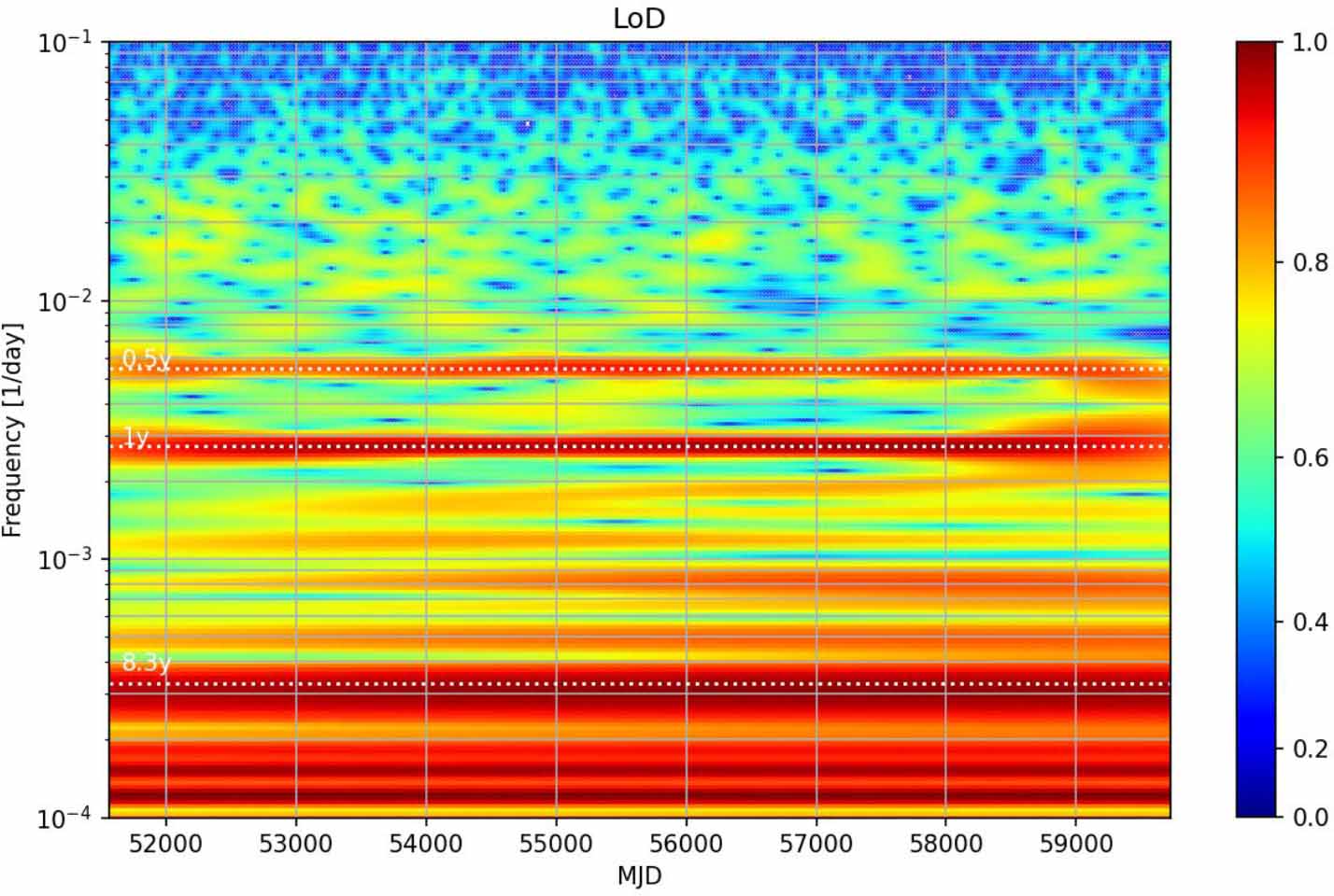
Figure 1.
Spectrogram for LOD
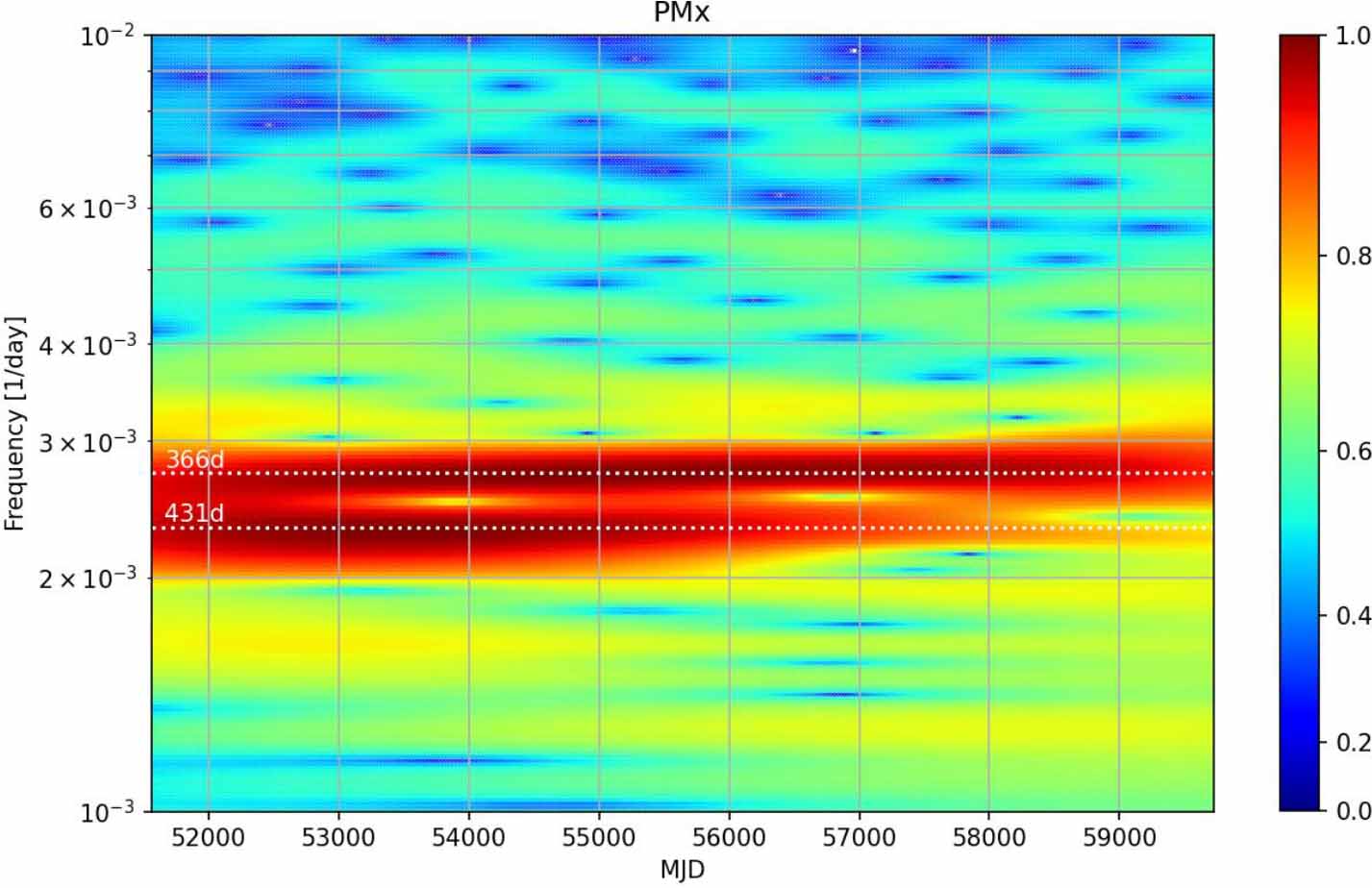
Figure 2.
Spectrogram for PMx
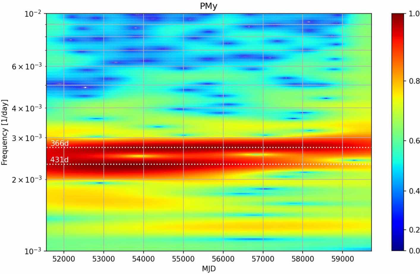
Figure 3.
Spectrogram for PMy
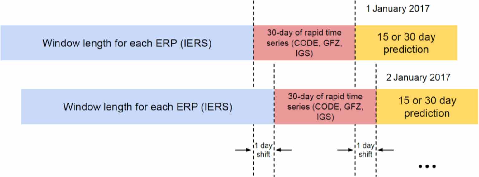
Figure 4.
Diagram of the whole prediction process with rapid products
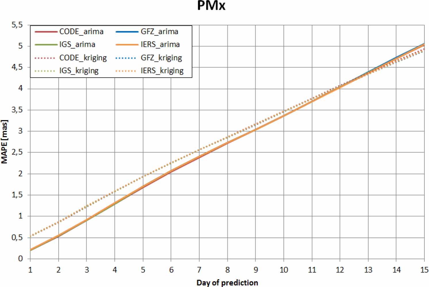
Figure 5.
Comparison of MAPEs for 15-day PMx prediction for ARIMA and kriging for various analysis centres (CODE, GFZ and IGS denote rapid time series and IERS final time series)
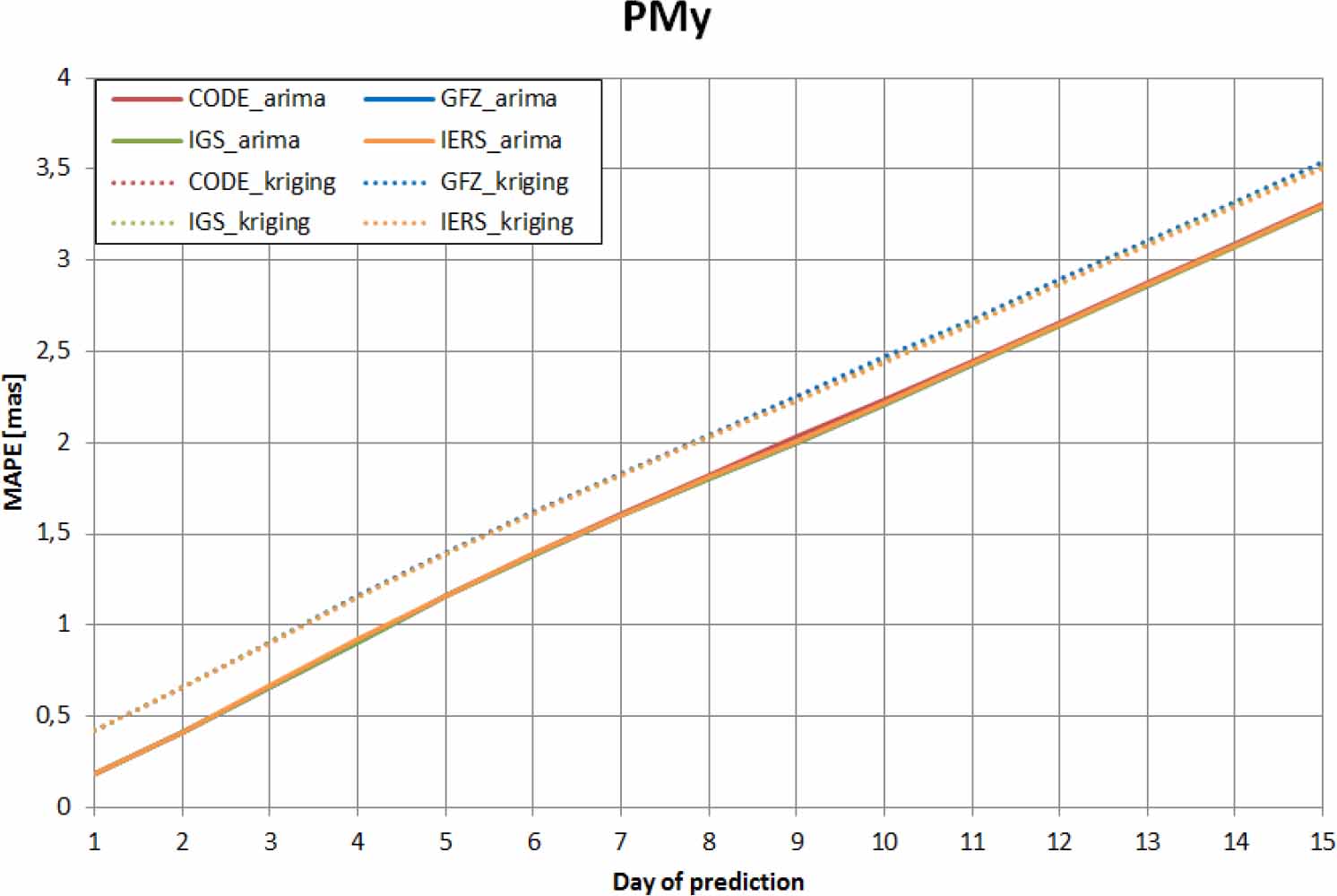
Figure 6.
Comparison of MAPEs for 15-day PMy prediction for ARIMA and kriging for various analysis centres
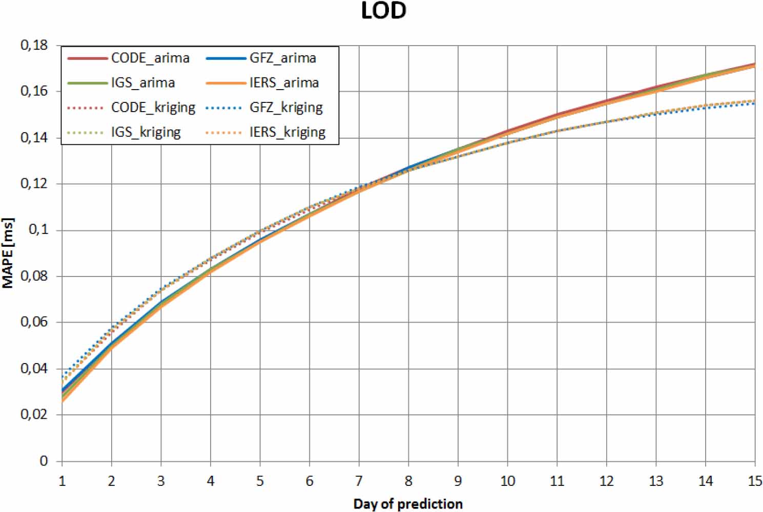
Figure 7.
Comparison of MAPEs for 15-day LOD prediction for ARIMA and kriging for various analysis centres
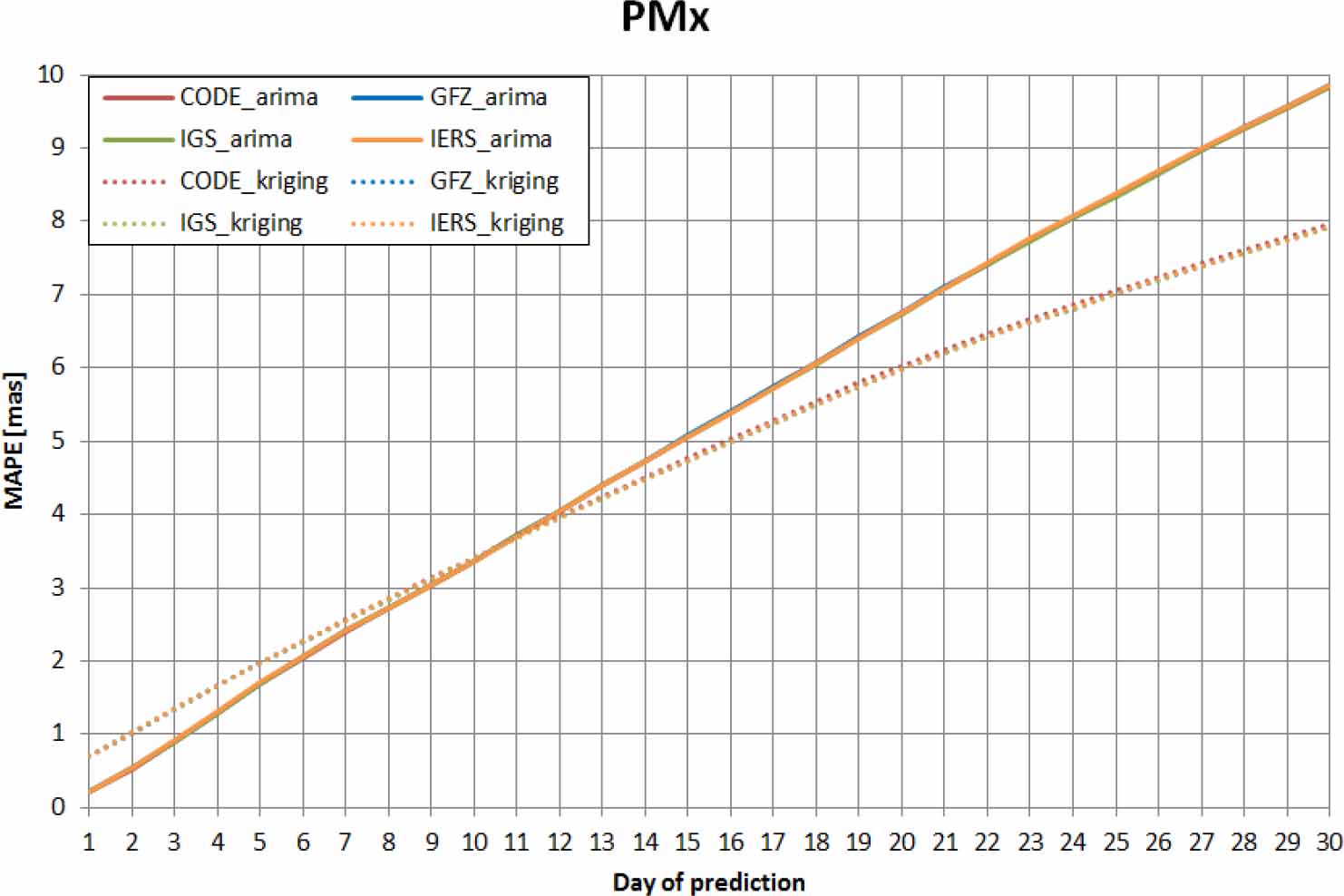
Figure 8.
Comparison of MAPEs for 30-day PMx prediction for ARIMA and kriging for various analysis centres
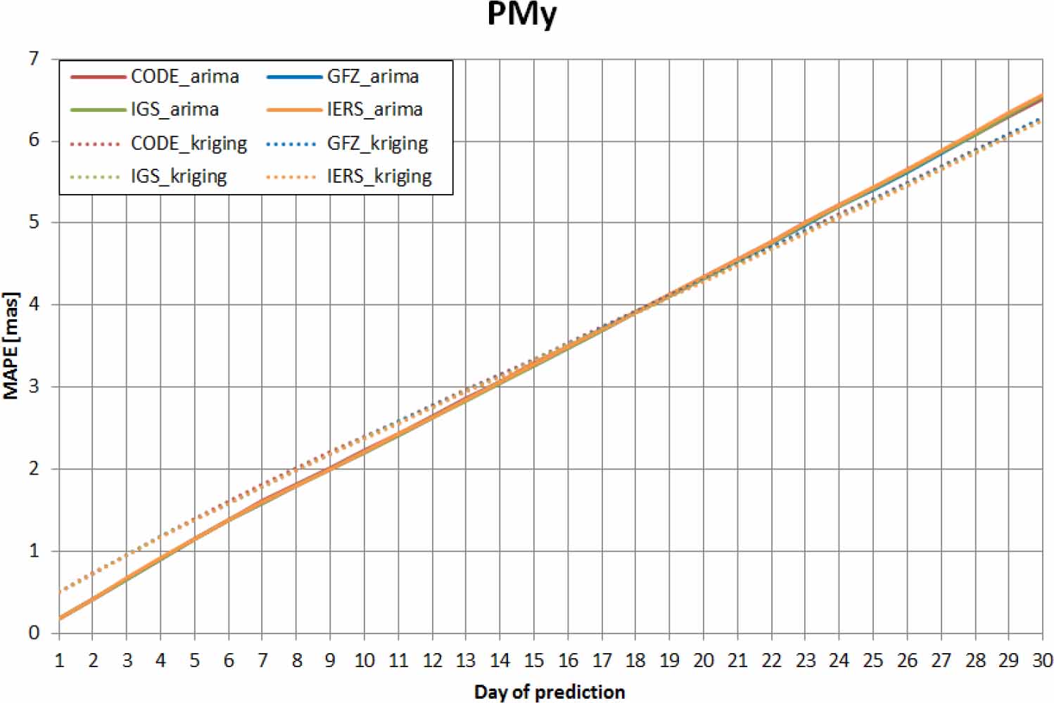
Figure 9.
Comparison of MAPEs for 30-day PMy prediction for ARIMA and kriging for various analysis centres
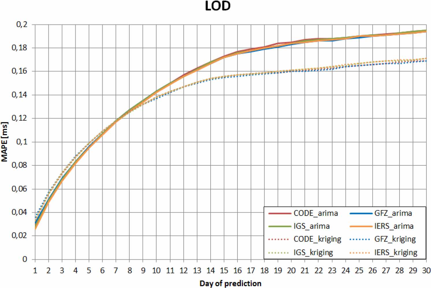
Figure 10.
Comparison of MAPEs for 30-day LOD prediction for ARIMA and kriging for various analysis centres