
For water authorities to effectively manage water reserves for different water users like hydropower generation, agricultural, domestic, flood management, etc., it is necessary to forecast river flow hours, days, months, or possibly longer in advance. Large volumes of dynamic, non-linear, and noisy data can be handled effectively using soft computing approaches, especially when the underlying physical relations are not understood.
For rainfall-runoff modeling and runoff forecasting, neural network models are successfully applied and can be found in the literature (Dawson & Wilby, 1998; Jain & Chalisgaonkar, 2000; Raghuwanshi, Singh & Reddy, 2006; Tayfur & Singh, 2006; Besaw, Rizzo, Bierman & Hackett, 2010; Rezaeian Zadeh, Amin, Khalili & Singh, 2010). The ASCE Task Committee (2000) reviews hydrologic applications of artificial neural network (ANN). Solaimani (2009) utilized ANN for modeling the rainfall runoff relationship in a catchment area located in a semiarid region of Iran by adopting feed forward back propagation for the rainfall forecasting with various algorithms with performance of multi-layer perceptions. The monthly stream flow of Jarahi watershed was analyzed to calibrate the given models. The monthly hydrometric and climatic were ranged from 1969 to 2000. The results extracted from the comparative study indicated that ANN was more appropriate and efficient to predict the river runoff than the classic regression model. Using the feed-forward back propagation neural network (FFBPNN) and the cascade forward back propagation neural network (CFBPNN) models, Mohseni and Muskula (2023) created rainfall-runoff-based models in the Yerli sub-catchment of the upper Tapi basin using data from 36 years from 1981 to 2016 and concluded that the developed ANN model was capable of predicting runoff quite accurately.
Wavelet transform (WT) has gained popularity recently as a helpful method for examining trends, periodicities, and variations in time series. Similar to the Fourier transform and short-time Fourier transform, a WT is a powerful mathematical tool for signal processing that can analyze both stationary and non-stationary data and produce time and frequency information at a higher resolution that is not possible with the former. The WT offers a multiresolution analysis; that is, at low scales (high frequency), it provides poor frequency resolution and better time resolution; at high scales (low frequency), it provides poor frequency resolution and higher time resolution. Such information is significant in real practice for all time-series signals. The WT breaks down a non-stationary time series into a specific number of stationary time series. The WT is then used to integrate other single prediction techniques to increase prediction accuracy. Another trustworthy hybrid model for application in time series forecasting issues is the wavelet-ANN (WANN). To estimate runoff discharge for the Ligvanchai watershed in Tabriz, Iran, Nourani, Komasi and Mano (2009) explored the rainfall-runoff modeling utilizing the wavelet-ANN technique. The time series were decomposed up to four levels using Haar, Daubechies (db2), Symlet (sym3), and Coiflet (coif1) wavelets. The model's outcomes demonstrated the great quality of the Haar wavelet when compared to the others. Kisi (2009b) proposed neuro-wavelet model for forecasting daily intermittent stream flow. Forecasting accuracy of neuro-wavelet model was better than single ANN model. To predict the flow of the Malbrabha river in India, Nayak, Venkatesh, Krishna and Jain (2013) developed a wavelet neural network (WNN) hybrid model employing the db5 wavelet for one time step ahead forecasting. According to the results, the WANN model outperformed the ANN model. Nourani, Baghanam, Adamowski and Gebremichael (2013) utilized feed forward neural networks (FFNN) to model the rainfall-runoff process on a daily and multi-step (two days, three days and four days) ahead time scale. Authors used db4 and Haar wavelets to remove noise from runoff time series and discovered that the performance of the FFNN was improved by applying WT to the raw runoff data. Also, it was concluded that db4 wavelet exhibits superior results as compared to Haar wavelet. Shafaei and Kisi (2017) compared the WANN model with ANN and SVM for prediction of short-term daily river flow of Ajichai river of Iran. A db5 mother wavelet was used to decompose the raw data and concluded that the WANN model performed better than ANN and SVM. Wang et al. (2022) developed hybrid models by combining the wavelet theory with five diverse types of machine learning models such as support vector machine (SVM)-radial basis function, SVM-polynomial, decision tree, gradient boosting, random forest, and long- or short-term memory. The db4 mother wavelet was used in the study. A comparison revealed that hybrid models exhibit better estimates than the stand-alone ones. To estimate monthly stream flows in Amasya, Turkey, Katipoǧlu (2023a) combined a discrete wavelet transform and a feedforward backpropagation neural network. The author decomposed various meteorological data using different wavelets such as Haar, Daubechies 2, Daubechies 4, Discrete Meyer, Coiflet 3, Coiflet 5, Symlet 3, and Symlet 5, and found that the results of Coiflet 5 was superior. Katipoǧlu (2023b) developed wavelet-ANFIS (W-ANFIS) model using db10 mother wavelet for predicting monthly Bitlis river flows in Turkey and concluded that the W-ANFIS model proved successful. Other studies on runoff prediction using wavelet-ANN are found in literature (Rao & Krishna, 2009; Adamowski & Sun, 2010; Linh et al., 2021; Kumar, Kumar, Kumar, Elbeltagi & Kuriqi, 2022). Nourani, Baghanam, Adamowski and Kisi (2014), Khandekar and Deka (2016) review the application of WT in hydrology. Application of WT in drought prediction, groundwater prediction, evaporation prediction can be found in the literature (Djerbouai & Souag-Gamane, 2016; Patil & Deka, 2017; Araghi, Adamowski & Martinez, 2020; Katipoǧlu, 2023c; Katipoǧlu, 2023d; Katipoǧlu, 2023e).
In time series forecasting issues, the wavelet-MLR (WMLR) is another trustworthy hybrid model. Kisi (2010) combined discrete wavelet transform and linear regression (WR) for short-term stream flow forecasting of two stations in Turkey. In comparison to ANN and ARMA models, WR models are found to be more superior. Kisi (2011) proposed a wavelet regression (WR) model for daily river stage forecasting of two stations on the Schuylkill river in Philadelphia. The result of a WR model was superior to the ANN models. Zhang, Zhang and Sing (2018) developed four models – MLR, ANN, wavelet coupled with MLR (W-MLR) and ANN (W-ANN) – for stream flow forecasting at four stations in the East River basin in China. All models showed similar performance in forecasting stream flow one-day ahead, while W-MLR and W-ANN performed better in five-day ahead forecasting. Other studies on runoff prediction using wavelet-MLR is found in literature (Kisi, 2009a; Budu, 2013; Shoaib et al., 2018; Khazaee Poul, Shourian & Ebrahimi, 2019).
Most previous investigations employed a selected mother wavelet type. Also, more research is required to fully understand the potential of Daubechies wavelets of different orders in studying hydrologic time series behavior. So, in this study, it is suggested to create hybrid models by coupling wavelet transform with ANN and MLR, with the following objectives:
To compare the results of all hybrid models (WANN, WMLR) developed using db1, db2, db3, db8 and db10 Daubechies wavelets for multiple lead times (two days, four days, seven days, 14 days). Also, to compare results of hybrid models with standalone ANN and MLR models.
To investigate the effect of Daubechies wavelets db1, db2, db3, db8, and db10 on forecasting accuracy.
To investigate how decomposition level affects model effectiveness.
With an average discharge at its mouth of 19,830 cumec, Brahmaputra is the fourth-largest river in the world (Goswami, 1985). Brahmaputra river Pancharatna station is selected for the study. Ten-year (Jan 1990 – Dec 1999) daily flow data were collected from Water Resources Department, Assam, India. The catchment area up to Pancharatna station is 532,000 km2. The seasonal monsoon rhythm and the Himalayan snow's freeze-thaw cycle influence the river's hydrologic regime. During the flood season, there are noticeable large changes in discharge over a short period of time. A maximum differential of roughly 17,000 m3·s−1 in 24 h (June 7–8, 1990) and 24,000 m3·s−1 in 48 h (June 7–9, 1990) was observed in rising limb (Sarma, 2005). The location of Pancharatna station is shown in Figure 1.
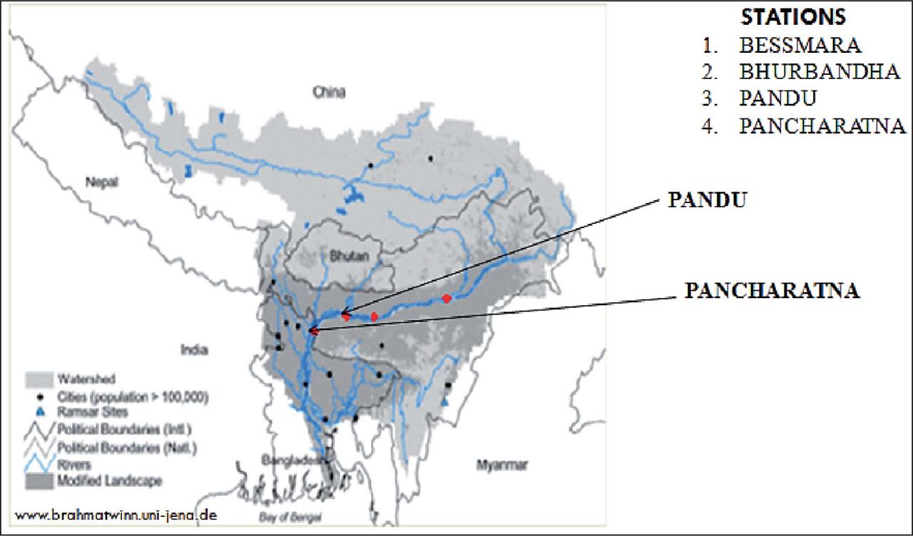
Location of the gauging sites
Source: Khandekar (2014)
Figure 2 displays the observed time series discharge at Pancharatna station. Figure 2 demonstrates that the discharge is remarkably non-stationary, particularly during monsoon season (from June to September, each year). The contribution of flow from snow melting, during February to April, causes the discharge in the rising limb to fluctuate as well.

Observed flow series
Source: Khandekar (2014)
Table 1 displays the statistical properties of flow data and demonstrates substantial variability. The terms Qmean, Qmax, Qmin, Sd, and Cx in the table stand for the mean, maximum, minimum, standard deviation, and skewness, respectively.
Statistical properties of flow data
| Statistical parameter | Training | Testing | All |
|---|---|---|---|
| Qmean [m3·s−1] | 16 159 | 16 236 | 16 161 |
| Qmax [m3·s−1] | 59 832 | 76 236 | 76 236 |
| Qmin [m3·s−1] | 2 628 | 1 723 | 1 723 |
| Sd [m3·s−1] | 11 783 | 12 388 | 11 965 |
| Cx | 0.726 | 0.968 | 0.809 |
Source: Khandekar (2014).
The discharge throughout the study period exhibits significant fluctuations, as shown in Table 1 (minimum = 1,723 cumec, the highest = 76,236 cumec). The standard deviation is determined to be 11,965 cumec, showing a significant dispersion of values from the mean. Additionally, the observed flows show significant positive coefficient of skewness (Cx = 0.809), indicating that the data has a more scattered distribution about the mean.
Wavelet theory is discussed thoroughly in works by Mallat (1998), and Labat, Ababou and Mangin (2000). Wavelet transform of a raw signal has the ability of providing time-frequency, using a range of window sizes. It divides the input signal into wavelets (small waves), which are scaled and shifted versions of the original wavelet, called mother wavelet. There are two forms of wavelet transformation: the continuous wavelet transform (CWT) and the discrete wavelet transform (DWT). The CWT of a signal x(t) is described:
In Eq. (1), the transformed signal is a function of two variables, a and b, which represent the scale and translation factor of the function ψ(t), respectively; * corresponds to complex conjugate (Mallat, 1998).
The ψ(t) is the transforming function, called as mother wavelet, is mathematically defined as:
From a data set of length (L), CWT produces L2 coefficients. Therefore, duplicate data is trapped within the coefficients, which may or may not be a desired quality (Nourani et al., 2009; Rajaee, Nourani, Zounemat-Kermani & Kisi, 2011). The analysis will be significantly more precise and efficient, resulting in N transform coefficients, if scales and positions are chosen based on the powers of two. The resulting transform is called DWT, and has the form:
Two sets of functions, known as high-pass (wavelet function) and low-pass (scaling function) filters, are operated by DWT. The original time series undergo processing via high-pass and low-pass filters (as shown in Fig. 3), followed by a down-sampled process that discards every second data point (Deka & Prahlada, 2012). The detailed (D1, D2, ..., Dn) and approximation (A1, A2, ..., An) coefficients, which represent the low frequency and high frequency components of the original signal, respectively, are derived after the signal is passed through high pass and low pass filters. There will be a total of n + 1 coefficients at every given nth decomposition level, where there will be one series of approximation coefficients at the nth level (An) and n series of detailed coefficients (D1, D2, ..., Dn). The sum of An + D1 + D2 +... + Dn is equal to the original signal.

Wavelet decomposition tree
Source: Khandekar (2014).
Neural networks are interconnected groups of artificial neurons that may be utilized as a computational model for information processing based on the connectionist approach to computing. An ANN may be thought of mathematically as a universal approximator with the capacity to learn from instances without the need of explicit physics.
Three-layer-feedforward artificial neural networks are most frequently utilized in hydrologic time series modeling (Jain & Chalisgaonkar, 2000; Raghuwanshi, Singh & Reddy, 2006; Tayfur & Singh, 2006; Bajirao, Kumar, Kumar, Elbeltagi & Kuriqi, 2021; Katipoǧlu, 2023a). In the current study, the Lavenberg–Marquardt (LM) learning function and tangent sigmoid as the transfer function were employed in the feedforward ANN. The LM technique was used to train the ANN since it is more effective and faster than the traditional gradient descent technique (Kisi, 2009b; Mohseni & Muskula, 2023). In three-layer-feedforward ANN, information flow takes place from the input to the output side. Weights regulate the strength of a signal that passes across connections between neurons, altering the information that is transferred between them. While not connected to nodes in the same layer, nodes in one layer are connected to those in the next one. As a result, a node's output in a layer depends exclusively on the inputs and weights it receives from the previous layers. Every node multiplies each input by its weight, adds up the result, and then runs the total through a transfer function to get the desired outcome. Typically, this transfer function is represented as a sigmoid function, which is an S-shaped curve that increases continuously. The “S” upper and lower limb attenuation keeps the raw sums smoothly within predetermined bounds. The transfer function additionally adds a nonlinearity that improves the network's capacity to represent complicated functions (Jain & Chalisgaonkar, 2000). The sigmoid function is monotonically growing, continuous, and differentiable everywhere.
The MLR is one of the statistical methods which represents a mathematical equation expressing the relation between two or more explanatory variable and a response variable. The MLR attempts to model the link between two or more explanatory variables and a response variable by fitting a linear equation to the observed data (Sharma, Isik, Srivastava & Kalin, 2013). The relationship between the dependent variable y and the independent variable x is described by the MLR equation as follows:
For deciding the number of input parameters, no fixed rule is available. The values of the future time step (Qt+n) in any time-series forecasting are inevitably reliant on the antecedent values Qt, Qt−1, Qt−2, …, Qt−j (Table 2). But because the value of j (lag) is not known beforehand, it is difficult to determine how many lags in the past will lead to higher efficiency. In hydrologic time series forecasting, determining j is crucial since it can help to reduce information loss and the omission of critical input variables that could interfere with training.
Correlation coefficients for the flow series
| Output* (Qt+n) | Input (Qt−j)* | |||||||||
|---|---|---|---|---|---|---|---|---|---|---|
| Qt | Qt−1 | Qt−2 | Qt−3 | Qt−4 | Qt−5 | Qt−6 | Qt−7 | Qt−8 | Qt−9 | |
| Qt+2 | 0.983 | 0.971 | 0.957 | 0.942 | 0.929 | 0.915 | 0.903 | 0.891 | 0.880 | 0.871 |
| Qt+4 | 0.957 | 0.942 | 0.928 | 0.915 | 0.902 | 0.891 | 0.880 | 0.870 | 0.862 | 0.854 |
| Qt+7 | 0.915 | 0.902 | 0.891 | 0.880 | 0.870 | 0.862 | 0.854 | 0.846 | 0.839 | 0.832 |
| Qt+14 | 0.846 | 0.839 | 0.832 | 0.825 | 0.818 | 0.812 | 0.805 | 0.799 | 0.792 | 0.784 |
n – lead time; j – lag.
Source: Khandekar (2014).
Numerous researchers (Sudheer, Gosain & Ramsastri, 2002; Budu, 2013; Nayak et al., 2013; Khazaee Poul et. al., 2019; Sun, Niu & Sivakumar, 2019; Katipoǧlu, 2023a, 2023b, 2023c) have used the technique based on the statistical features such as cross-correlation, autocorrelation and partial correlation of the data series in order to identify a distinct input vector. In the current research, based on the autocorrelation coefficient between the relevant variables (shown in Table 2), the input vectors to the models are chosen. To forecast the value of discharge, based on the following various input combinations were taken into account (Khandekar, 2014):
Qt.
Qt, Q(t−1).
Qt, Q(t−1), Q(t−2).
Qt, Q(t−1), Q(t−2), Q(t−3).
Qt, Q(t−1), Q(t−2), Q(t−3), Q(t−4).
Qt, Q(t−1), Q(t−2), Q(t−3), Q(t−4), Q(t−5).
At the first stage, to forecast discharge, ANN and MLR models without data preprocessing were created. In the present study it was decided to predict discharge for multiple lead times such as two days, four days, seven days and 14 days because the Brahmaputra river is one of the major rivers in India which carries heavy flood during monsoon season, so it is necessary to design flood warning system well in advance. First 70% data was used to train the model and last 30% data was used for testing the model. Initially, a three-layer feedforward backpropagation ANN were applied in the study. For each lead time, an optimal input combination is obtained by providing each of one to six input combination obtained through autocorrelation as input to ANN and by varying number of neurons in the hidden layer from two to 10 through trial and error (Budu, 2013; Moosavi, Vafakhah, Shirmohammadi & Behnia, 2013). The optimal input combination that gave the minimum root mean square error (RMSE) during testing period for each lead time is shown in Table 3. The output layer has only one neuron which is the discharge value for the given lead time. From viewpoint of comparing all models, same input combination is employed for the MLR and all hybrid models. The time series data normalized between zero and one (Nourani et al., 2009) by dividing the discharge value by the maximum one.
Optimal input combination
| Lead time [day] | Input parameter* | Output parameter** Q(t+n) |
|---|---|---|
| 2 | Qt, Q(t−1) | Q(t+2) |
| 4 | Qt, Q(t−1), Q(t−2), Q(t−3) | Q(t+4) |
| 7 | Qt, Q(t−1), Q(t−2), Q(t−3) | Q(t+7) |
| 14 | Qt, Q(t−1), Q(t−2), Q(t−3) | Q(t+14) |
Qt – current discharge value; Q(t−1), Q(t−2), Q(t−3) – one-, two- and three-time step past discharge values;
n – lead time.
Source: Khandekar (2014).
After developing the ANN and MLR models, hybrid models were developed. First of all, using DWT, for developing hybrid models, the normalized input data were decomposed into approximation and detail coefficients. Since all hydrological data are observed at discrete time intervals, all hybrid models used DWT to process time series data in the form of approximations and details at various levels so that gross and small features of a signal can be separated (Deka & Prahlada, 2012). Then, to obtain the output at a predetermined lead time, the approximation and detail coefficient were fed as input to ANN and MLR. Without decomposition, the output signals were preserved as normalized original series. The complete flow chart of model development is shown in Figure 4.
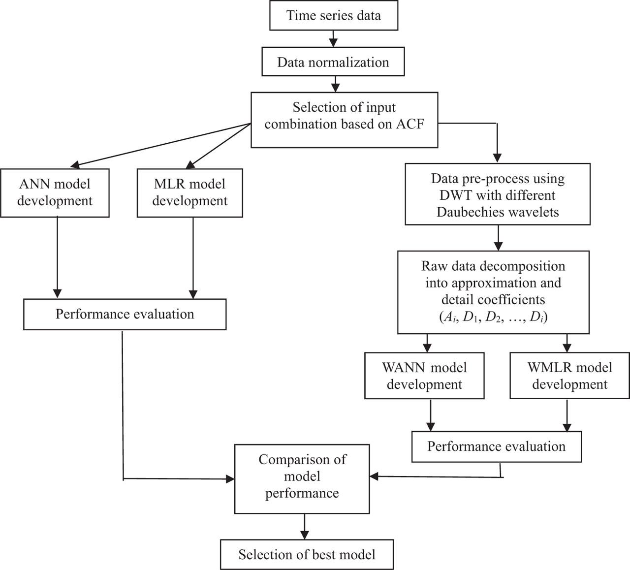
Flow chart of model development
Source: own elaboration.
The mother wavelet that will be used depends on the data to be analyzed (Nayak et al., 2013). As per authors' knowledge, there is no comparative study on prediction of hydrological parameter using group of Daubechies wavelets. So, in this research, an irregular wavelet, Daubechies (db) of orders 1 (db1), 2 (db2), 3 (db3), 8 (db8), and 10 (db10), illustrated in Figure 5, was chosen to deal with very irregular signal form. Daubechies wavelets of order N (dbN) are all asymmetric, orthogonal, and biorthogonal. They are compactly supported wavelets with extremal phase and highest number of vanishing moments for a given support width (Misiti, Misiti, Oppenheim & Poggi, 2010). Daubechies wavelet has a support width of 2N – 1. Except for db1 (haar), no Daubechies wavelet has an explicit expression. Wavelets with compact support or a narrow window function are appropriate for a local analysis of the signal.
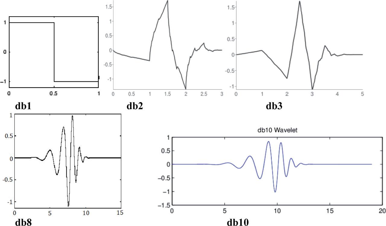
Daubechies wavelets
Source: Khandekar (2014).
The optimal decomposition level was obtained using the formula l = int [log (L)], (Nourani et al., 2014; Khazaee et al., 2019; Tarate et al., 2021; Katipoǧlu, 2023a, 2023b, 2023c), where l is the decomposition level, L represents the number of time series data, int represents the integer part function, and log represents logarithm with base 10. In the present study, L is 3,650 so l is approximately four. However, in our study, we decomposed raw signal up to fifth level. At any lth decomposition level, DWT produces l detailed coefficients and one approximation coefficient at lth level.
The following evaluation measures were used to compare model performance.
The results of all models are presented in Tables 4–7. It can be seen from Tables 4–7 that in comparison with MLR models, the ANN model has performed better for all lead times, except for the fourteen-day one. It is observed that the effectiveness of both models decreases while increasing lead time. This could be due to considerable fluctuations in the data around mean values, such as a high standard deviation. Tables 4–7 also indicates the optimal ANN structure (e.g. for a two-day lead time, 2-8-1 means two neurons in the input layer, eight neurons in the hidden layer, and one neuron in the output layer).
Values of statistical parameters for two-day lead time
| Model type | Training period | Testing period | Optimum ANN structure | ||||||||
|---|---|---|---|---|---|---|---|---|---|---|---|
| RMSE | R2 | MAE | BIAS | SI | RMSE | R2 | MAE | BIAS | SI | – | |
| ANN | 1 764.66 | 0.977 | 1 044.28 | 1.002 | 0.109 | 2 463.33 | 0.960 | 1 401.83 | 1.014 | 0.152 | 2-8-1 |
| MLR | 1 828.26 | 0.976 | 1 058.12 | 1.000 | 0.113 | 2 535.96 | 0.958 | 1 293.19 | 1.000 | 0.156 | – |
| WANN-db1l5 | 1 199.43 | 0.989 | 757.47 | 1.008 | 0.074 | 1 795.99 | 0.979 | 1 144.51 | 1.018 | 0.110 | 12-2-1 |
| WMLR-db1l5 | 1 228.25 | 0.989 | 680.19 | 1.000 | 0.076 | 1 758.64 | 0.980 | 913.41 | 1.000 | 0.109 | – |
| WANN-db2l4 | 960.30 | 0.993 | 540.14 | 1.001 | 0.059 | 1 415.36 | 0.987 | 796.43 | 1.007 | 0.087 | 10-2-1 |
| WMLR-db2l5 | 1 093.66 | 0.991 | 595.74 | 1.000 | 0.068 | 1 478.74 | 0.986 | 769.43 | 0.999 | 0.091 | – |
| WANN-db3l4 | 813.84 | 0.995 | 469.56 | 1.001 | 0.050 | 1 202.33 | 0.990 | 698.70 | 1.007 | 0.074 | 10-3-1 |
| WMLR-db3l5 | 909.81 | 0.994 | 510.23 | 1.000 | 0.056 | 1 311.38 | 0.989 | 629.76 | 0.999 | 0.081 | – |
| WANN-db8l5 | 553.07 | 0.998 | 368.93 | 1.000 | 0.034 | 1 054.10 | 0.992 | 543.92 | 1.000 | 0.065 | 12-2-1 |
| WMLR-db8l5 | 526.83 | 0.998 | 296.78 | 1.000 | 0.033 | 775.11 | 0.996 | 406.20 | 0.999 | 0.048 | – |
| WANN-db10l5 | 481.40 | 0.998 | 298.51 | 0.999 | 0.030 | 933.06 | 0.994 | 436.49 | 0.999 | 0.057 | 12-2-1 |
| WMLR-db10l5 | 471.99 | 0.998 | 261.79 | 1.000 | 0.029 | 751.87 | 0.996 | 369.69 | 1.000 | 0.046 | – |
Note: MAE and RMSE are m3·s−1 unit (Results of only optimum decomposition level are shown).
Source: own elaboration.
Values of statistical parameters for four-day lead time
| Model type | Training period | Testing period | Optimum ANN structure | ||||||||
|---|---|---|---|---|---|---|---|---|---|---|---|
| RMSE | R2 | MAE | BIAS | SI | RMSE | R2 | MAE | BIAS | SI | ||
| ANN | 3 133.09 | 0.929 | 2 067.41 | 1.005 | 0.194 | 3 890.35 | 0.901 | 2 566.07 | 1.031 | 0.239 | 4-8-1 |
| MLR | 3 136.83 | 0.929 | 1 988.84 | 1.000 | 0.194 | 3 932.06 | 0.899 | 2 274.72 | 1.000 | 0.243 | – |
| WANN-db1l5 | 1 918.22 | 0.973 | 1 229.16 | 1.008 | 0.118 | 2 590.84 | 0.956 | 1 717.58 | 1.018 | 0.159 | 24-3-1 |
| WMLR-db1l5 | 2 088.67 | 0.968 | 1 268.59 | 1.000 | 0.129 | 2 909.44 | 0.945 | 1 618.86 | 1.000 | 0.179 | – |
| WANN-db2l5 | 1 431.04 | 0.985 | 868.66 | 1.001 | 0.088 | 1 986.38 | 0.974 | 1 137.20 | 1.009 | 0.122 | 24-2-1 |
| WMLR-db2l4 | 1 922.49 | 0.973 | 1 160.03 | 1.000 | 0.119 | 2 342.13 | 0.964 | 1 354.14 | 0.999 | 0.144 | – |
| WANN-db3l5 | 1 280.06 | 0.988 | 790.25 | 1.001 | 0.079 | 1 683.59 | 0.982 | 1 034.97 | 1.004 | 0.104 | 24-2-1 |
| WMLR-db3l5 | 1 528.75 | 0.983 | 924.38 | 1.000 | 0.094 | 2 067.67 | 0.972 | 1 084.63 | 0.999 | 0.127 | – |
| WANN-db8l4 | 962.64 | 0.993 | 601.76 | 1.001 | 0.059 | 1 465.35 | 0.986 | 774.11 | 1.000 | 0.090 | 20-2-1 |
| WMLR-db8l5 | 940.03 | 0.994 | 556.62 | 1.000 | 0.058 | 1 213.32 | 0.990 | 664.47 | 0.999 | 0.075 | – |
| WANN-db10l5 | 822.67 | 0.995 | 527.85 | 1.003 | 0.051 | 1 477.12 | 0.986 | 755.19 | 1.004 | 0.091 | 24-2-1 |
| WMLR-db10l5 | 785.37 | 0.995 | 460.22 | 1.000 | 0.048 | 1 174.80 | 0.991 | 612.69 | 1.000 | 0.072 | – |
Note: MAE and RMSE are in m3·s−1 unit (Results of only optimum decomposition level are shown).
Source: own elaboration.
Values of statistical parameters for seven-day lead time
| Model type | Training period | Testing period | Optimum ANN structure | ||||||||
|---|---|---|---|---|---|---|---|---|---|---|---|
| RMSE | R2 | MAE | BIAS | SI | RMSE | R2 | MAE | BIAS | SI | ||
| ANN | 4 308.72 | 0.866 | 2 801.05 | 1.002 | 0.266 | 5 185.33 | 0.825 | 3 441.99 | 1.032 | 0.318 | 4-3-1 |
| MLR | 4 490.92 | 0.854 | 2 986.84 | 1.000 | 0.277 | 5 376.87 | 0.811 | 3 429.75 | 0.999 | 0.331 | – |
| WANN-db1l5 | 2 830.19 | 0.942 | 1 961.30 | 1.004 | 0.175 | 4 131.69 | 0.889 | 2 942.38 | 1.016 | 0.254 | 24-3-1 |
| WMLR-db1l5 | 3 122.62 | 0.929 | 1 942.73 | 1.000 | 0.193 | 4 123.65 | 0.889 | 2 415.44 | 0.999 | 0.254 | – |
| WANNdb2l5 | 2 038.56 | 0.970 | 1 408.02 | 1.004 | 0.126 | 2 894.02 | 0.945 | 1 927.13 | 1.024 | 0.178 | 24-2-1 |
| WMLR-db2l5 | 2 623.55 | 0.950 | 1 617.63 | 1.000 | 0.162 | 3 193.40 | 0.933 | 1 937.76 | 0.999 | 0.196 | – |
| WANN-db3l5 | 1 683.52 | 0.979 | 1 151.42 | 1.003 | 0.104 | 2 525.32 | 0.958 | 1 639.74 | 1.013 | 0.155 | 24-3-1 |
| WMLR-db3l5 | 2 129.55 | 0.967 | 1 336.34 | 1.000 | 0.132 | 2 987.57 | 0.942 | 1 640.06 | 0.999 | 0.184 | – |
| WANN-db8l5 | 1 313.63 | 0.987 | 871.91 | 0.999 | 0.081 | 2 038.33 | 0.973 | 1 233.97 | 0.997 | 0.125 | 24-2-1 |
| WMLR-db8l5 | 1 318.74 | 0.987 | 837.08 | 1.000 | 0.082 | 1 702.96 | 0.981 | 1 042.41 | 0.999 | 0.105 | – |
| WANN-db10l5 | 1 187.51 | 0.989 | 792.06 | 0.999 | 0.073 | 1 929.58 | 0.975 | 1 060.01 | 1.005 | 0.119 | 24-2-1 |
| WMLR-db10l5 | 1 167.65 | 0.990 | 733.49 | 1.000 | 0.072 | 1 585.02 | 0.984 | 881.76 | 1.000 | 0.097 | – |
Note: MAE and RMSE are in m3·s−1 unit (Results of only optimum decomposition level are shown).
Source: own elaboration.
Values of statistical parameters for 14-day lead time
| Model type | Training period | Testing period | Optimum ANN structure | ||||||||
|---|---|---|---|---|---|---|---|---|---|---|---|
| RMSE | R2 | MAE | BIAS | SI | RMSE | R2 | MAE | BIAS | SI | ||
| ANN | 5 704.97 | 0.765 | 4 035.67 | 1.014 | 0.353 | 7 084.21 | 0.673 | 5 116.37 | 1.068 | 0.433 | 4-2-1 |
| MLR | 4 584.37 | 0.848 | 3 204.37 | 1.000 | 0.283 | 5 415.77 | 0.809 | 3 630.94 | 0.999 | 0.333 | – |
| WANN-db1l5 | 4 173.09 | 0.874 | 2 765.27 | 1.007 | 0.258 | 4 913.55 | 0.843 | 3 425.92 | 1.036 | 0.300 | 24-4-1 |
| WMLR-db1l5 | 4 761.19 | 0.836 | 3 215.26 | 1.000 | 0.294 | 6 050.48 | 0.762 | 3 886.88 | 0.999 | 0.371 | – |
| WANN-db2l5 | 3 071.96 | 0.932 | 2 062.78 | 1.004 | 0.190 | 4 716.30 | 0.855 | 3 017.38 | 1.038 | 0.288 | 24-3-1 |
| WMLR-db2l5 | 4 037.44 | 0.882 | 2 571.67 | 1.000 | 0.249 | 4 876.84 | 0.845 | 3 109.41 | 0.999 | 0.299 | – |
| WANN-db3l5 | 2 420.95 | 0.958 | 1 737.07 | 1.014 | 0.149 | 3 848.56 | 0.904 | 2 663.88 | 1.031 | 0.235 | 24-2-1 |
| WMLR-db3l5 | 3 172.17 | 0.927 | 2 083.46 | 1.000 | 0.196 | 4 770.31 | 0.852 | 2 694.26 | 0.999 | 0.292 | –– |
| WANN-db8l5 | 1 922.74 | 0.973 | 1 353.08 | 1.012 | 0.119 | 3 746.15 | 0.908 | 2 190.53 | 1.020 | 0.229 | 24-2-1 |
| WMLR-db8l5 | 1 985.33 | 0.971 | 1 325.19 | 1.000 | 0.123 | 2 612.09 | 0.955 | 1 731.46 | 0.999 | 0.160 | – |
| WANN-db10l5 | 2 225.74 | 0.964 | 1 600.63 | 0.995 | 0.138 | 3 539.60 | 0.918 | 2 287.83 | 0.986 | 0.217 | 24-3-1 |
| WMLR-db10l5 | 1 670.31 | 0.979 | 1 137.67 | 1.000 | 0.103 | 2 196.46 | 0.968 | 1 435.57 | 1.000 | 0.134 | – |
Note: MAE and RMSE are in m3·s−1 unit (Results of only optimum decomposition level are shown).
Source: own elaboration.
The normalized observed data was decomposed using Daubechies wavelets of order 1 (db1), 2 (db2), 3(db3), 8 (db8) and 10 (db10) up to fifth level decomposition, which were fed as input to ANN and MLR, making the models as WANN(dbNli) and WMLR(dbNli), respectively, where N is the order of Daubechies wavelet and i is decomposition level. The performances of these hybrid models only for best decomposition level (low RMSE) are presented in Tables 4–7. Results of Tables 4–7 show that wavelet-based hybrid models perform significantly better than the standalone model.
After comparing the results of hybrid models with respect to wavelet order, it was observed that all models' efficiency is increasing with wavelet order, highest being at 10th order. For example, for four-day lead time (during testing period), from the Table 4 it was found that for WANN model the value of R2 increased from 0.956 (WANN-db1l5) to 0.986 (WANN-db10l5) and for WMLR model the increase is from 0.945 (WMLR-db1l5) to 0.991 (WMLR-db10l5). Similar trend was observed for all lead times. Table 8 shows percent improvement in RMSE values with increase in Daubechies wavelet order from db1 to db10. The average percent improvement in RMSE is found to be 57.19%. Figure 6 shows a sample plot of effect of Daubechies wavelet order on RMSE for four-day lead time.
Percent improvement in RMSE with increase in wavelet order from db1 to db10
| Lead time [day] | Improvement in RMSE [%] |
|---|---|
| 2 | 57.25 |
| 4 | 54.66 |
| 7 | 61.56 |
| 14 | 55.30 |
Source: own elaboration.
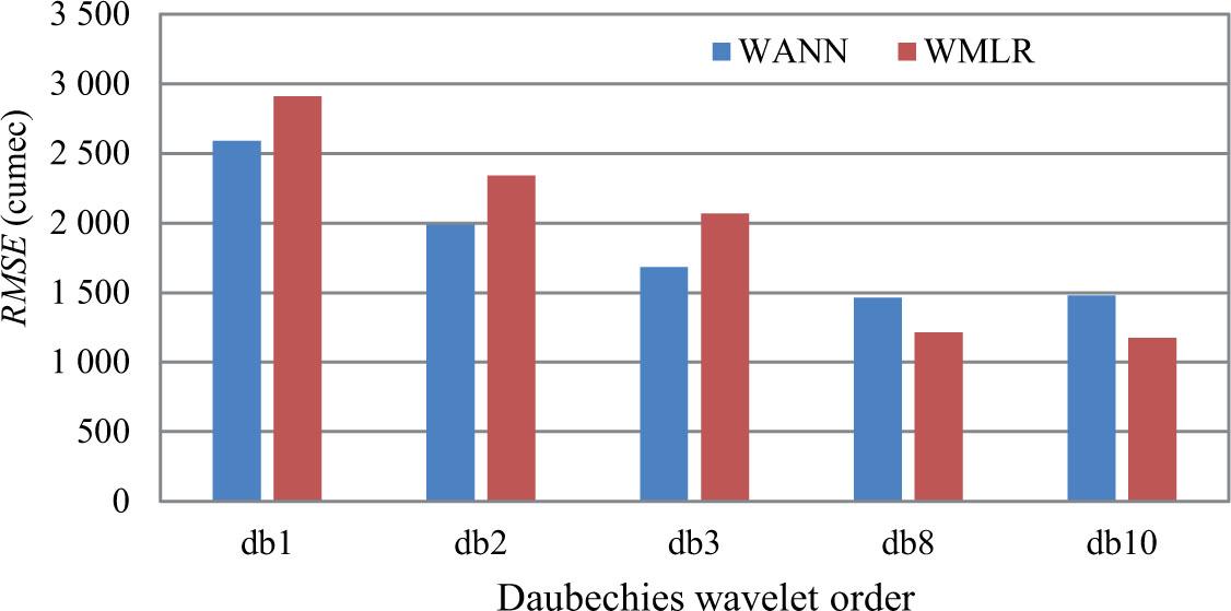
Effect of Daubechies wavelet order on RMSE (four-day lead time)
Source: own elaboration.
In general, for all lead times, from the analysis it was found that for lower order wavelets (db1, db2, db3), WANN model performance was better as compared to the WMLR model, while for higher order wavelets (db8, db10), WMLR was found to be superior as compared to WANN. A careful study of Tables 4–7 reveals that the forecasting ability of each hybrid model improves with increasing wavelet order. According to the observed time series flow data (Fig. 2), it appears to occur in a high frequency during the monsoon season (June to September, i.e. four months out of the year) and in a low frequency during the other non-monsoon eight months. Wider-support wavelets can capture low frequencies, while wavelets with a smaller support can capture high frequencies. The support width of a Daubechies wavelet of order N is equal to 2N – 1 (Misiti et al., 2010), hence the support widths of db1, db2, db3, db8, and db10, wavelets are one, three, five, 15, and 19, respectively. In brief, compared to db1, db2, db3, and db8 wavelet-based forecast models, the db10 wavelet has a reasonable support and good time-frequency localization properties, which together allow the model to capture both the underlying trend and the short-term variations in the time series. This conclusion is consistent with the findings of (Nourani et al., 2013; Katipoǧlu, 2023b, 2023e), who demonstrated that higher order mother wavelet (db4 and db10) offered substantially better results than lower order Haar (db1) wavelet. Scatter plots for all lead times for best model [WMLR(db10)] are shown in Figure 7. The scatter plots showed that the majority of the points were quite close to the 45° line, with only a few having greater magnitudes of observed flow on the lower side, indicating model underestimate (BIAS slightly below 1.0). WMLR(db10) models performance was very satisfactory (R2 > 0.9) (Dawson & Wilby, 2001) for all lead times. Time series plots are shown in Figure 8 for all lead times.

Scatter plot for lead time during different testing period
Source: own elaboration.
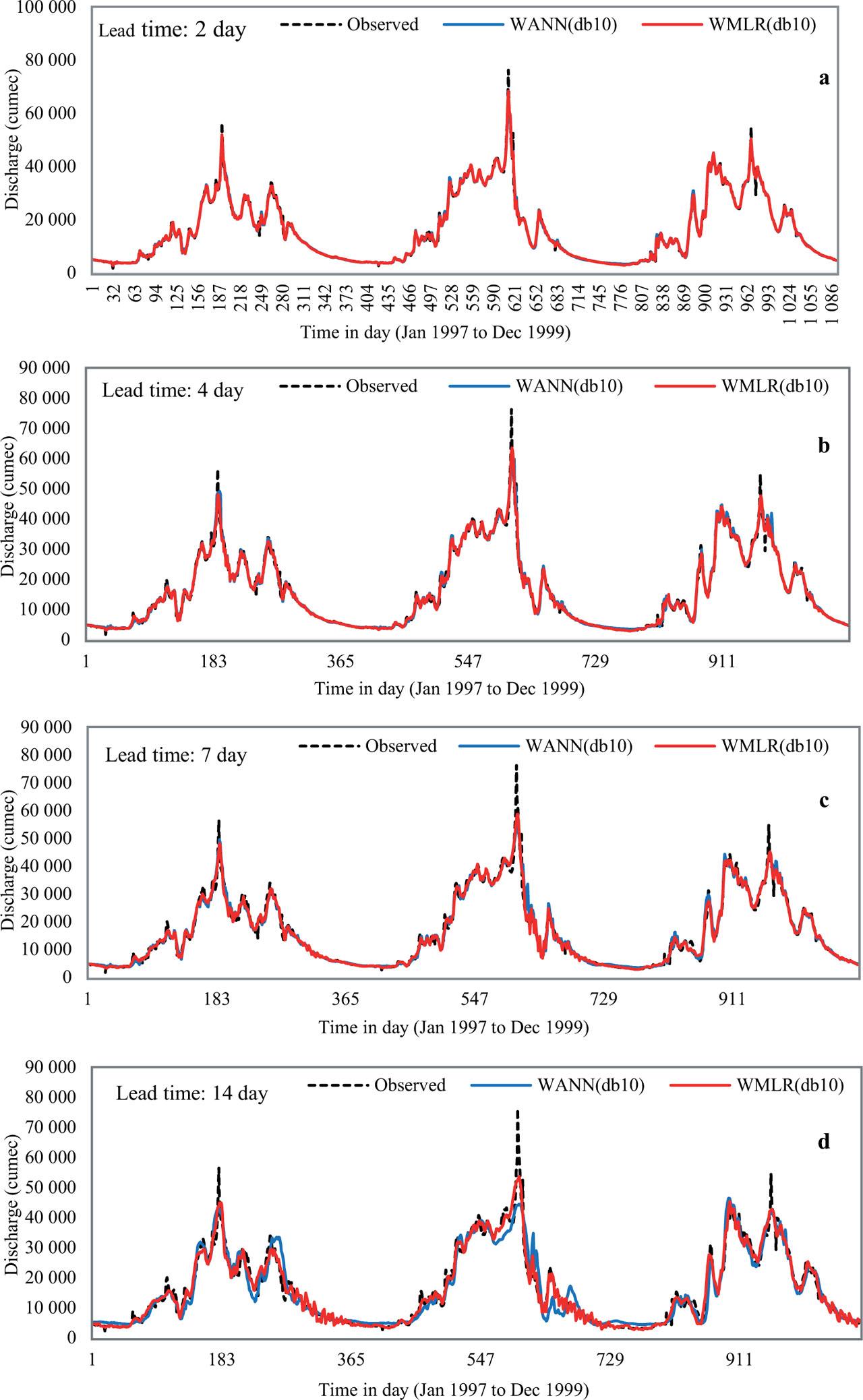
Time series plot for lead time during different testing period influence of decomposition level on model performance
Source: own elaboration.
As mentioned earlier, the optimum decomposition level was determined using the formula l = int [log (L)]. In our study, we decomposed raw signal up to fifth level. For the best model WMLR(db10), the effect of decomposition level on R2 is presented in Table 9. A careful examination of Table 9 demonstrates that model efficiency enhances with decomposition level. The initial resolution level of the original time series captures the high frequency components, and as the decomposition level (scale) is increased, the signal becomes smoother and more stationary. As a result, prediction errors were not affected by scale. Figure 9 shows effect of decomposition level on R2 for WMLR(db10) model for all lead times.
Effect of decomposition level on determination coefficient (R2) for WMLR-db10 model (testing period)
| Two-day lead time | Four-day lead time | Seven-day lead time | 14-day lead time | ||||
|---|---|---|---|---|---|---|---|
| Model type | R2 | Model type | R2 | Model type | R2 | Model type | R2 |
| WMLR-db10l1 | 0.976 | WMLR-db10l1 | 0.914 | WMLR-db10l1 | 0.824 | WMLR-db10l1 | 0.656 |
| WMLR-db10l2 | 0.995 | WMLR-db10l2 | 0.966 | WMLR-db10l2 | 0.861 | WMLR-db10l2 | 0.684 |
| WMLR-db10l3 | 0.996 | WMLR-db10l3 | 0.990 | WMLR-db10l3 | 0.967 | WMLR-db10l3 | 0.760 |
| WMLR-db10l4 | 0.996 | WMLR-db10l4 | 0.991 | WMLR-db10l4 | 0.983 | WMLR-db10l4 | 0.953 |
| WMLR-db10l5 | 0.996 | WMLR-db10l5 | 0.991 | WMLR-db10l5 | 0.984 | WMLR-db10l5 | 0.968 |
Source: own elaboration.
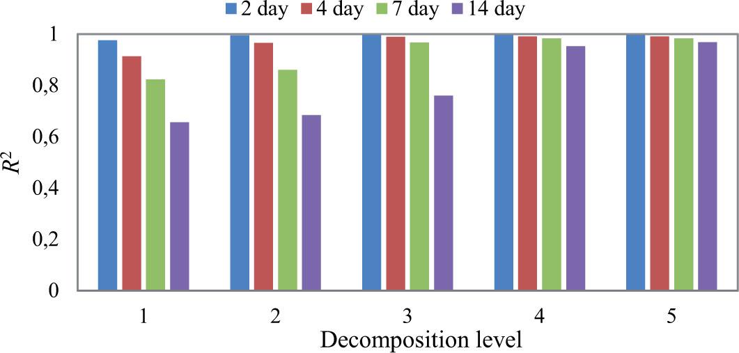
Effect of decomposition level on determination coefficient (R2) for WMLR(db10) model
Source: own elaboration.
Finally, because the Brahmaputra river carries substantial flood during the monsoon season (June to September), an attempt was made to assess the model's accuracy during the monsoon period (for three years in testing from 1997 to 1999) for the WMLR(db10) model. The statistical parameter values for the WMLR(db10) model during testing period of monsoon season are shown in Table 10. As shown in Table 10, the WMLR(db10) model demonstrated good performance during monsoon season producing extremely satisfactory results for all lead times, despite substantial non-stationarity. Figure 10 compares flow series between observed, WMLR(db10) and WANN(db10) modelled flow for monsoon season for two-day lead time. From Figure 10 it is clear that the WMLR(db10) model has captured well almost all peaks, except the highest.
Values of statistical parameters for WMLR(db10) model for monsoon season (June to September) in testing period
| Year | RMSE | R2 | MAE | BIAS | S.I. |
|---|---|---|---|---|---|
| Two-day lead time | |||||
| 1997 | 890.55 | 0.995 | 596.966 | 1.000 | 0.034 |
| 1998 | 1 448.88 | 0.995 | 767.802 | 0.999 | 0.042 |
| 1999 | 1 070.20 | 0.996 | 629.899 | 0.999 | 0.034 |
| Four-day lead time | |||||
| 1997 | 1 572.65 | 0.984 | 1 072.41 | 1.000 | 0.059 |
| 1998 | 2 188.39 | 0.989 | 1 153.71 | 0.999 | 0.063 |
| 1999 | 1514.68 | 0.992 | 968.89 | 0.998 | 0.048 |
| Seven-day lead time | |||||
| 1997 | 2 243.79 | 0.967 | 1 667.90 | 0.998 | 0.084 |
| 1998 | 2 971.27 | 0.980 | 1 677.60 | 1.001 | 0.086 |
| 1999 | 1 797.46 | 0.989 | 1 209.73 | 0.999 | 0.058 |
| 14-day lead time | |||||
| 1997 | 3 035.86 | 0.938 | 2 292.43 | 1.002 | 0.115 |
| 1998 | 3 722.21 | 0.967 | 2 295.27 | 1.006 | 0.111 |
| 1999 | 2 588.93 | 0.976 | 1 972.25 | 0.998 | 0.084 |
Note: RMSE and MAE are in cumec unit.
Source: own elaboration.

Flow series comparison between observed, WMLR(db10) and WANN(db10) modelled flow for monsoon season
Source: own elaboration.
In this study, hybrid models were created by coupling wavelet transform with ANN and MLR to predict the Brahmaputra River flow at Pancharatna station for two-, four-, seven-, and 14-day lead time using 10-year daily flow data. Daubechies wavelets db1, db2, db3, db8, and db10 were used to decompose the observed raw flow data up to fifth level, which were used as input to ANN and MLR. After comparing the results of WANN and WMLR models with respect to wavelet order, it was found that both hybrid models' efficiency is increasing with wavelet order, highest being at 10th order. Comparing the hybrid models' outcomes, it was discovered for all lead times that the WMLR-db10 model had produced more reliable and superior results than the WANN model. The average percent improvement in RMSE with increase in wavelet order from one to 10 was found to be 57.19%. Also, it was concluded that with increase in the decomposition level the model's efficiency was increased. Finally, it was concluded that the wavelet transform as a preprocessing tool has proved to be best for mapping the relation between input and output as compared to a single model. To evaluate the forecasting effectiveness of suggested wavelet coupled hybrid models, other hydrological time series variables, such as rainfall, temperature, and evapotranspiration, can be employed as model inputs. To investigate more accuracy, the work can be expanded with additional wavelet types. Study can further be applied at other stations with highly non-stationary data.