
Table 1.
Primers used to compare M. aegracyperi n. sp. with its closest relatives.
| Primer | Sequence (5′-3′) | Use | Marker |
|---|---|---|---|
| D2A | ACAAGTACCGTGAGGGAAAGTTG | PCR and sequencing | 18S rRNA |
| D2B | TCGGAAGGAACCAGCTACTA | PCR and sequencing | 18S rRNA |
| ITS1 | CGTAACAAGGTAGCTGTAG | PCR and sequencing | ITS rRNA |
| ITS2 | TTTCACTCGCCGTTACTAAGG | PCR and sequencing | ITS rRNA |
| 1618 F | TTT GTA CAC AC GCC CGT CG | Sequencing | 18S rRNA |
| 1421 F deg | GGT CTG TGA TGC CCT WRG ATG T | Sequencing | 18S rRNA |
| 546 F | GGG CAA GTC TGG TGC CAG CAG | Sequencing | 18S rRNA |
| Nema 28 S R AG | ACT CCT TGG TCC GTG TTT CAA GA | PCR | 18S rRNA |
| 983 F deg | CGA MRG YGA TYA GAT ACC GCY | PCR | 18S rRNA |
| 1629 R deg | GGT GTG TAC AAA KSR CAG GGA | PCR | 18S rRNA |
| 79 F deg | GDG AAACYG CGWACG GCT | PCR | 18S rRNA |
| RKN-5R | TCG AAC ATG TCA AAA GGA GC | PCR and sequencing | HSP90 |
| RKN-d1F | GCY GAT CTT GTY AAC AAC CYT GGA AC | PCR and sequencing | HSP90 |
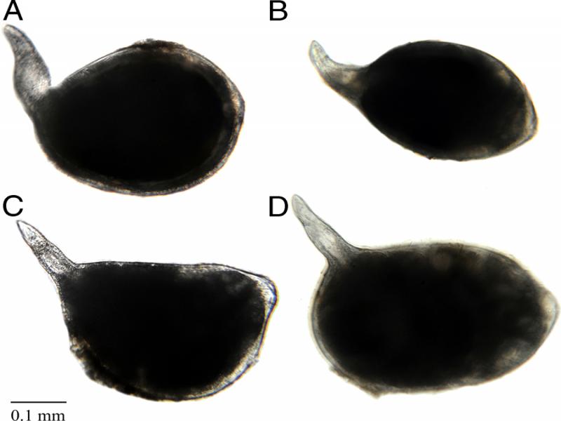
Figure 1:
Females of Meloidogyne aegracyperi n. sp.; (A-D) Light micrographs of whole specimens showing the typical shape of the body and the posterior protuberance containing the perineal pattern (scale bar=0.1 mm).
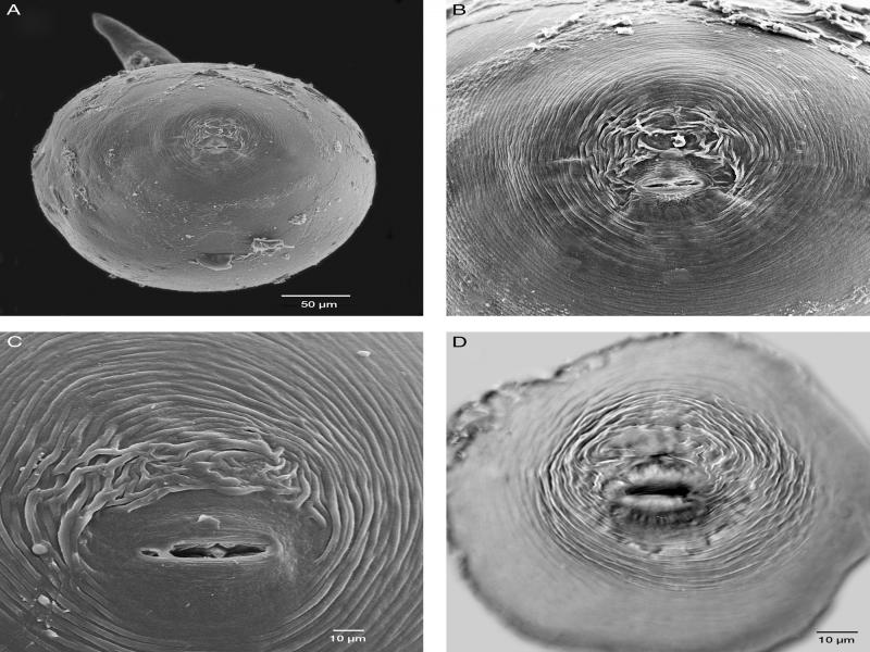
Figure 2:
Scanning electron (SEM) and light micrographs of females of Meloidogyne aegracyperi n. sp.; (A) SEM of a whole female showing the location of the perineal pattern; (B) SEM of a perineal pattern situated on a protuberance of the posterior end of the body (magnification same as Fig. D); (C) SEM close-up of a perineal pattern; (D) Light micrograph showing the protuberance of the posterior end of the body containing the perineal pattern as seen in Fig. B.
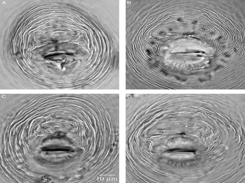
Figure 3:
Light micrographs of perineal patterns of females of Meloidogyne aegracyperi n. sp.
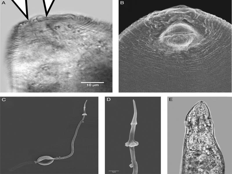
Figure 4:
Light (LM) and scanning electron micrographs (SEM) of females of Meloidogyne aegracyperi n. sp.; (A) LM of posterior protuberance containing the perineal pattern with the anus and vulva marked by arrows; (B) SEM of posterior protuberance showing the swollen vulval lips and tail terminus; (C) SEM of the extracted cuticular lining of the esophagus with the stylet and showing the triradiate plates of the metacorpus and the vesicles in the lumen lining that are usually contained in the anterior region of the metacorpus; (D) SEM of an extracted stylet showing the angular edges on the knobs and the long dorsal esophageal gland orifice; (E) LM of the anterior end of the female showing the stylet and metacorpus.
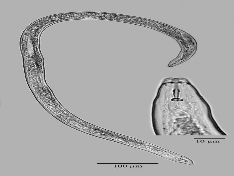
Figure 5:
Light micrographs of a whole male specimen with an enlarged view of the anterior end of Meloidogyne aegracyperi n. sp.
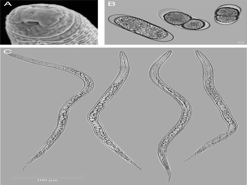
Figure 6:
(A) Scanning electron micrograph of the anterior end of a second-stage juvenile of Meloidogne aegracyperi n. sp. (B) Light micrographs (LM) of eggs of M. aegracyperi n. sp. showing the variation in size for three eggs in the two-cell stage. Light micrographs of second-stage juveniles of M. aegracyperi n. sp.
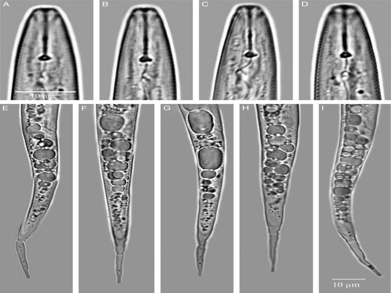
Figure 7:
Light micrographs of the anterior ends and tails of second-stage juveniles of Meloidogyne aegracyperi n. sp.
Table 2.
Measurements and ratios of Meloidogyne aegracyperi n. sp. females, males, and second-stage juveniles.
| Female | Male | Second-stage Juv. | ||
|---|---|---|---|---|
| Character | Holotype | Paratypes | Paratypes | Paratypes |
| N | – | 30 | 2 | 30 |
| L | 360 | 373 ± 44 | 1124 ± 10.5 | 426 ± 24.7 |
| – | (310–460) | (1113–1134) | (388–484) | |
| Body diam. | 292 | 306 ± 46 | 30.9 ± 1.4 | 15 ± 0.9 |
| – | (210–420) | (29.5–32.3) | (13.6–17.4) | |
| Neck length | 148 | 153 ± 27 | – | – |
| – | (100–210) | – | – | |
| Stylet length | 12 | 12 ± 0 | 15.6 ± 1.0 | 10.9 ± 0.4 |
| – | (12–12) | (14.6–16.5) | (10.1–11.8) | |
| Stylet knob height | 1.5 | 1.5 ± 0.2 | 2.3 ± 0.2 | 1.4 ± 0.2 |
| – | (1.2–1.9) | (2–2.5) | (1.1–1.9) | |
| Stylet knob width | 2.4 | 2.6 ± 0.3 | 4.1 ± 0.1 | 2.1 ± 0.2 |
| – | (2–3) | (4–4.2) | (1.7–2.5) | |
| DGO | 4.8 | 4.8 ± 0.6 | 3.1 ± 0.1 | 3.7 ± 0.5 |
| – | (4–6.1) | (3.0–3.3) | (2.7–4.8) | |
| Stylet tip to metacorpus center | 60.1 | 63.8 ± 2.2 | – | – |
| – | (59–67) | – | – | |
| Interphasmidial distance | – | 18 ± 2.7 | – | – |
| – | (14.2–24.4) | – | – | |
| Vulva length | – | 21 ± 2.9 | – | – |
| – | (13.5–26) | – | – | |
| Vulva-anus distance | – | 15.7 ± 2.3 | – | – |
| – | (10.9–21) | – | – | |
| Ant. end to excretory pore | – | – | 94.7 ± 1.6 | 68.5 ± 7.9 |
| – | – | (93.1–96.3) | (52–80.4) | |
| Tail length | – | – | 12.7 ± 1.9 | 73.1 ± 4.9 |
| – | – | (10.8–14.5) | (63.6–88.7) | |
| Body width at anus | – | – | – | 11 ± 0.6 |
| – | – | – | (10.2–11.9) | |
| a | 1.3 | 1.2 ± 0.2 | – | 28.4 ± 2.8 |
| – | (0.8–1.7) | – | (23.6–34.6) | |
| c | – | – | – | 5.8 ± 0.4 |
| – | – | – | (5.1–6.5) | |
| Spicule length | – | – | 23.6 ± 1.8 | – |
| – | – | (21.8–25.4) | – | |
| Hyaline tail terminus | – | – | – | 22 ± 2.0 |
| – | – | – | (18.5–26.6) | |
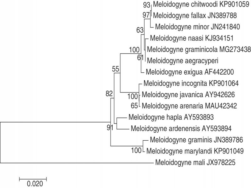
Figure 8:
Maximum likelihood phylogenetic analysis of evolutionary relationships of closely related Meloidogyne species including NSRKN (Meloidogyne aegracyperi n. sp.) and comparison 18S rRNA sequences. The tree with the highest log likelihood (−2,286.9884) is shown. The bootstrap support values (500 bootstraps) are shown at nodes next to the branches. Branch lengths are proportional to the distances. Genbank accession numbers follow each species.
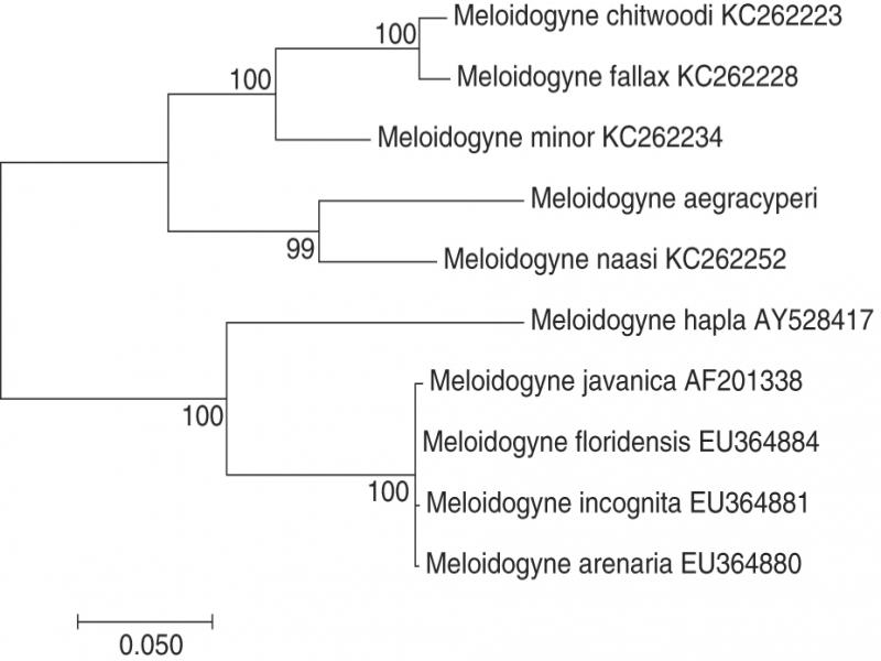
Figure 9:
Maximum likelihood phylogenetic analysis of evolutionary relationships of closely related Meloidogyne species including NSRKN (Meloidogyne aegracyperi n. sp.) and comparison Hsp90 sequences. The tree with the highest log likelihood (−2,926.7701) is shown. The bootstrap support values (500 bootstraps) are shown next to the branches. Branch lengths are proportional to the distances. Genbank accession numbers follow each species.
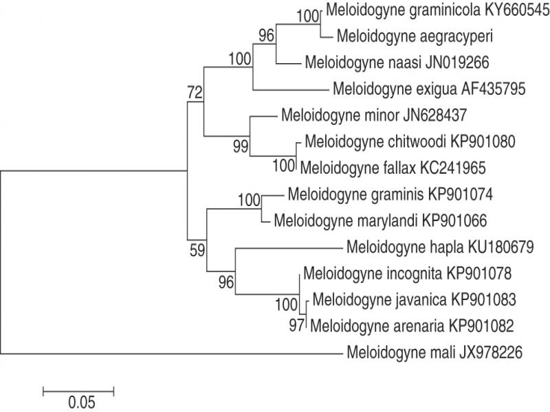
Figure 10:
Maximum likelihood phylogenetic analysis of evolutionary relationships of closely related Meloidogyne species including Meloidogyne aegracyperi n. sp. and comparison of the alignment of the D2-D3 (28S rRNA) sequences. The tree with the highest log likelihood is shown. The bootstrap support values (500 bootstraps) are shown at nodes next to the branches. Branch lengths are proportional to the distances. Genbank accession numbers follow each species.
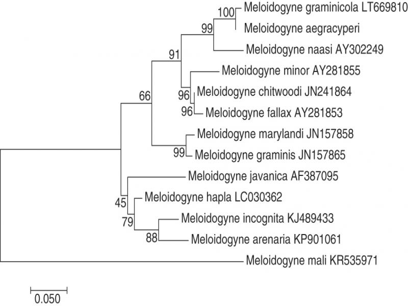
Figure 11:
Maximum likelihood phylogenetic analysis of evolutionary relationships of closely related Meloidogyne species including Meloidogyne aegracyperi n. sp. and comparison of the alignment of the ITS sequences. The tree with the highest log likelihood is shown. The bootstrap support values (500 bootstraps) are shown at nodes next to the branches. Branch lengths are proportional to the distances. Genbank accession numbers follow each species.
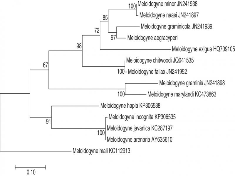
Figure 12:
Maximum likelihood phylogenetic analysis of evolutionary relationships of closely related Meloidogyne species including Meloidogyne aegracyperi n. sp. and comparison of the alignment of the COII-16S rRNA sequences. The tree with the highest log likelihood is shown. The bootstrap support values (500 bootstraps) are shown at nodes next to the branches. Branch lengths are proportional to the distances. Genbank accession numbers follow each species.
Table 3.
Comparisons of key measurements of females, second-stage juveniles, and males of Meloidogyne aegarcyperi n. sp. with its closest-related species: M. graminicola Golden and Birchfield, 1965; M. naasi Franklin, 1965; M. fallax Karrsen, 1996; M. minor Karssen, Bolk, van den Beld, Kox, Korthals, Molendijk, Zijlstra, van Hood, and Cook, 2004; and M. chitwoodi Golden, O'Bannon, Santo, and Finley, 1980.
| Female | |||||
| Species | Length | Width | Stylet | DGO | Vulva |
| M. chitwoodi (n=60)a | (430–750) 591 | (344–518) 422 | (11.2–12.5) 11.9 | (3.4–5.5) 4.2 | |
| M. fallax (n=30)b | (404–720) 491 | (256–464) 362 | (13.9–15.2) 14.5 | (3.8–6.3) 4.3 | (20.2–28.4) 24.7 |
| M. minor (n=25)c | (416–608) 526 | (240–464) 339 | (12.6–15.2) 14.2 | (3.2–6.3) 4.1 | (22.8–29.1) 25.8 |
| M. naasi (n=25)d | (455–705) 557 | (227–398) 330 | (11–15) 13 | (2–4) 3 | (17–25) 22 |
| M. graminicola (n=20)e | (455–765) 573 | (275–520) 419 | (10.6–11.2) 11.1 | (2.8–3.9) 3.2 | |
| M. aegracyperi n. sp. (n=30) | (310–460) 373 | (210–420) 306 | (12–12) 12 | (4–6.1) 4.8 | (13.5–26) 21 |
| Juvenile | |||||
| Species | Length | Stylet | DGO | Tail | Terminus |
| M. chitwoodi (n=60)a | (336–417) 390 | (9.0–10.3) 9.9 | (2.6–3.9) 3.2 | (39–47) 43 | (8.6–13.8) 11 |
| M. fallax (n=30)b | (381–435) 403 | (10.1–11.4) 10.8 | (3.2–3.8) 3.5 | (46.1–55.6) 49.3 | (12.2–15.8) 13.5 |
| M. minor (n=25)c | (310–416) 377 | (7.6–10.1) 9.2 | (3.2–4.4) 3.8 | (58.1–77.1) 54 | (12.0–22.1) 16.1 |
| M. naasi (n=25)d | (418–465) 435 | (13–15) 14 | (2–3) 2.4 | (52–78) 70 | 17.5 |
| M. graminicola (n=20)e | (415–484) 441 | (11.2–12.3) 11.4 | (2.8–3.4) 2.8 | (67.0–76.0) 70.9 | (14.0–21.2) 17.9 |
| M. aegracyperi n. sp. (n=30) | (388–484) 426 | (10.1–11.8) 10.8 | (2.7–4.8) 3.7 | (63.6–88.7) 73.1 | (18.5–26.6) 22 |
| Male | |||||
| Species | Stylet | DGO | |||
| M. chitwoodi (n–30)a | (18.1–18.5)18.3 | (2.2–3.4) 3 | |||
| M. fallax (n=30)b | (18.9–20.9) 19.6 | (3.2–5.7) 4.4 | |||
| M. minor (n=25)c | (17.1–19.0) 17.8 | (3.2–4.4) 3.8 | |||
| M. naasi (n=25)d | (16–19) 18 | (2–4) 3 | |||
| M. graminicola (n=20)e | (16.2–17.4) 16.8 | (2.8–3.9) 3.3 | |||
| M. aegracyperi n. sp. (n= 2) | (14.6–16.5) 15.6 | (3.0–3.3) 3.1 | |||
1 Length = maximum body length; Width = maximum body width; Stylet = maximum stylet length; DGO = length of the dorsal gland orifice to the base of the stylet knobs; Vulva = maximum width of the vulva; Tail = distance from the anus to the tail tip; Terminus = distance of the hyaline portion of the tail to the tip of the tail.
2 a Golden et al. (1980); b Karssen (1996); c Karssen et al. (2004); d Franklin (1965); eGolden and Birchfield (1965).
Table 4.
Hosts and non-host plants of Meloidogyne aegracyperi n. sp. compared to eight populations of its closest-related species: M. graminicola Golden and Birchfield, 1965 (Minton et al., 1987; Soomro and Hague, 1992a,b); and M. naasi Franklin, 1965, reported by Franklin (1965) from the type population in England; Radewald et al. (1970) and Allen et al. (1970) from California; and Michell et al. (1973) from England, California, Illinois, Kansas, and Kentucky.
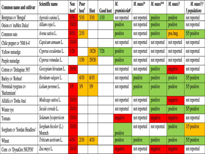
1 August 13, 2008 - planted and inoculated with 5,000 per pot.
*Franklin, 1965;**Radewald et al., 1970; †Allen et al., 1970; and ‡Michell et al., 1973 tested populations from England, California, Illinois, Kansas, and Kentucky; aProportion of 10 plants that exhibited host characteristics; bpoor host = RF (ratio of eggs recovered/inoculum level) > 0 but < 1; host = RF > 1 but < 10; good host = RF > 10; red = non or poor host, yellow = non and good host, and green = good host.