
Table 1.
Means and standard errors (SD) of the soil physical properties, microbial respiration, microbial biomass carbon, and enzymes in different ecosystems: forest F; forest with F. japonica FF; grassland G; grassland with F. japonica GF; wetland W; wetland with F. japonica WF.
| F | FF | G | GF | W | WF | ||||||||||||||
|---|---|---|---|---|---|---|---|---|---|---|---|---|---|---|---|---|---|---|---|
| Soil Indices | H | Mean | SD | Mean | SD | Mean | SD | Mean | SD | Mean | SD | Mean | SD | ||||||
| Soil moisture (%) | 21.93*** | 9.1 | 0.04 | c | 14.0 | 0.55 | ab | 9.5 | 0.35 | ac | 11.7 | 0.06 | abc | 12.4 | 0.94 | abc | 21.5 | 0.98 | b |
| Soil pH (CaCl2) | 22.30*** | 5.2 | 0.06 | a | 6.4 | 0.06 | ab | 6.1 | 0.06 | ac | 6.8 | 0.06 | ab | 6.8 | 0.05 | bc | 7.2 | 0.06 | b |
| Soil microbial respiration | 21.86*** | 139.6 | 7.37 | abc | 185.1 | 8.14 | bc | 58.0 | 14.67 | a | 123.5 | 7.28 | abc | 90.4 | 15.30 | ad | 147.8 | 14.84 | bcd |
| Microbial biomass carbon | 17.18** | 344.0 | 33.52 | ab | 370.6 | 11.99 | a | 289.9 | 10.93 | b | 297.5 | 12.6 | b | 309.5 | 8.59 | ab | 351.0 | 16.15 | ab |
| Urease | 35.15***,1 | 1.5 | 0.03 | a | 1.3 | 0.02 | ab | 1.2 | 0.11 | ab | 1.4 | 0.08 | a | 0.9 | 0.26 | b | 0.6 | 0.04 | b |
| Acid phosphatase | 21.79*** | 60.0 | 1.43 | a | 53.1 | 2.78 | ab | 58.2 | 0.75 | ac | 57.5 | 1.00 | ab | 34.1 | 4.24 | bc | 24.1 | 1.54 | b |
| Alkaline phosphatase | 21.37*** | 26.1 | 0.65 | b | 38.3 | 1.18 | ab | 31.7 | 4.57 | ab | 44.2 | 1.31 | a | 34.4 | 2.23 | ab | 26.2 | 0.73 | b |
| Invertase | 27.80***,2 | 39.9 | 1.13 | c | 33.9 | 2.91 | ac | 21.2 | 0.99 | b | 25.5 | 0.77 | ab | 31.1 | 1.20 | ab | 28.2 | 0.28 | ab |
1 Note: H means statistics H (5, N = 24) from Kruskal–Wallis test (For 1N = 42 and for 2N = 30). Significant differences from multiple post hoc comparisons of site characteristics between ecosystems are indicated by different lowercase letters (a,b,c,d) in every row with p less than 0.05. Significance level: ***0.001; **0.001 levels, respectively.
Table 2.
List of identified nematode species and their mean abundance in ind./100 g of soil (n = 5) and standard errors (SD) in different ecosystems: forest F; forest with F. japonica FF; grassland G; grassland with F. japonica GF; wetland W; wetland with F. japonica WF; c-p value of colonizer–persister nematode species from 1 to 5 according to Bongers (1990).
| F | FF | G | GF | W | WF | |||||||||
|---|---|---|---|---|---|---|---|---|---|---|---|---|---|---|
| Nematode species/trophic groups | Abbr. | c-p | Mean | SD | Mean | SD | Mean | SD | Mean | SD | Mean | SD | Mean | SD |
| Bacterivores | ||||||||||||||
| Acrobeles cylindricus (Ivanova, 1968) | Acyl | 2 | – | – | – | – | 3.6 | 5.7 | – | – | 0.2 | 0.4 | – | – |
| Acrobeloides nanus (de Man, 1880) | Anan | 2 | 5.4 | 5.0 | 3.0 | 1.9 | 2.6 | 3.4 | 11.2 | 9.5 | 18.4 | 9.4 | 5.0 | 5.5 |
| Alaimus primitivus (de Man, 1880) | Apri | 4 | 9.6 | 2.9 | 2.2 | 1.1 | 2.2 | 3.2 | 4.0 | 3.1 | 7.0 | 5.0 | 0.6 | 0.9 |
| Cephalobus persegnis (Bastian, 1865) | Cper | 2 | 0.8 | 1.8 | – | – | 9.6 | 8.6 | 1.8 | 1.8 | 14.6 | 14.4 | 3.2 | 4.0 |
| Cervidellus vexilliger (de Man, 1880) | Cvex | 2 | 3.6 | 4.3 | – | – | – | – | 1.4 | 2.1 | – | – | – | – |
| Eucephalobus oxyuroides (de Man, 1876) | Eoxy | 2 | – | – | – | – | 0.8 | 1.8 | – | – | – | – | – | – |
| Eucephalobus striatus (Bastian, 1865) | Estr | 2 | – | – | 1.0 | 1.4 | 6.4 | 4.8 | 0.4 | 0.9 | 6.8 | 5.2 | 6.2 | 7.1 |
| Chiloplacus propinquus (de Man, 1921) | Cpro | 2 | 0.6 | 1.3 | 0.4 | 0.5 | 0.2 | 0.4 | 1.0 | 0.7 | 0.4 | 0.9 | 0.2 | 0.4 |
| Mesorhabditis sp. juv. | Msp. | 1 | 0.4 | 0.9 | – | – | – | – | – | – | – | – | – | – |
| Panagrolaimus rigidus (A. Schneider, 1866) | Prig | 1 | – | – | – | – | – | – | – | – | 0.2 | 0.4 | 0.8 | 1.3 |
| Plectus parietinus (Bastian, 1865) | Ppar | 2 | 5.0 | 6.2 | 0.4 | 0.9 | 1.4 | 2.1 | 0.2 | 0.4 | 4.8 | 3.6 | 1.0 | 1.2 |
| Plectus parvus (Bastian, 1865) | Ppai | 2 | 3.8 | 3.4 | 1.6 | 2.5 | 5.4 | 3.9 | 3.0 | 2.2 | 7.8 | 6.1 | 4.0 | 3.3 |
| Plectus tenuis (Bastian, 1865) | Pten | 2 | 0.2 | 0.4 | – | – | 1.2 | 2.7 | – | – | – | – | – | – |
| Prismatolaimus dolichurus (de Man, 1880) | Pdol | 3 | – | – | – | – | 2.8 | 3.9 | – | – | – | – | – | – |
| Prismatolaimus intermedius (Bütschli, 1873) | Pint | 3 | 58.8 | 59.0 | 7.8 | 11.7 | 4.2 | 3.3 | 6.2 | 4.1 | 3.6 | 2.3 | 1.0 | 1.2 |
| Punctodora sp. juv. | Psp. | 3 | 0.6 | 1.3 | – | – | – | – | – | – | – | – | – | – |
| Rhabditis spp. juv. | Rspp | 1 | 27.8 | 18.0 | 39.4 | 17.3 | 37.4 | 24.5 | 77.6 | 33.0 | 146.6 | 104.5 | 38.8 | 26.4 |
| Teratocephalus terrestris (Bütschli, 1873) | Tter | 3 | 2.6 | 2.1 | 2.6 | 3.6 | 1.8 | 2.7 | 1.4 | 2.6 | – | – | – | – |
| Wilsonema schuurmansstekhoveni (de Coninck, 1931) | Wsch | 2 | 2.6 | 4.2 | 2.2 | 2.3 | 0.8 | 1.3 | 4.4 | 4.3 | 0.6 | 0.9 | 1.2 | 2.2 |
| Fungivores | ||||||||||||||
| Aphelenchoides composticola (Franklin, 1957) | Acom | 2 | 0.2 | 0.4 | 0.6 | 0.9 | 2.2 | 3.2 | 1.4 | 2.1 | 0.6 | 0.5 | – | – |
| Aphelenchoides minimus (Meyl, 1953) | Amin | 2 | 0.2 | 0.4 | – | – | 3.6 | 3.8 | 0.4 | 0.5 | – | – | – | – |
| Aphelenchoides ritzemabosi (Schwartz, 1911) | Arit | 2 | – | – | – | – | 0.6 | 1.3 | 0.2 | 0.4 | 3.4 | 4.6 | 2.4 | 1.9 |
| Aphelenchus avenae (Bastian, 1865) | Aave | 2 | – | – | 0.6 | 0.9 | 6.2 | 3.9 | 6.0 | 6.4 | 19 | 29.1 | 4.0 | 3.8 |
| Doryllium zeelandicum (de Man, 1876) | Dzee | 4 | – | – | 0.2 | 0.4 | 4.4 | 6.2 | 5.2 | 9.5 | 7.6 | 11.2 | 1.2 | 1.8 |
| Tylencholaimus stecki (Steiner, 1914) | Tste | 4 | – | – | – | – | 4.0 | 8.4 | – | – | – | – | – | – |
| Omnivores | ||||||||||||||
| Aporcelaimellus obtusicaudatus (Bastian, 1865) | Aobt | 5 | – | – | – | – | 0.4 | 0.9 | – | – | – | – | – | – |
| Axonchium coronatum (de Man, 1906) | Acor | 5 | – | – | – | – | – | – | 0.4 | 0.5 | – | – | – | – |
| Diphtherophora communis (de Man, 1880) | Dcom | 3 | – | – | – | – | 8.2 | 8.8 | – | – | 26.2 | 21.9 | 2.2 | 2.9 |
| Enchodelus macrodorus (de Man, 1880) | Emac | 4 | 1.4 | 1.9 | 0.6 | 1.3 | 13.6 | 6.8 | – | – | – | – | 1.0 | 1.4 |
| Eudorylaimus silvaticus (Brzeski, 1960) | Espp | 4 | 10.8 | 6.0 | 1.4 | 1.7 | 7.4 | 2.7 | 1.2 | 1.1 | 9.0 | 7.0 | 6.0 | 4.7 |
| Eudorylaimus spp. juv. | Esil | 4 | 7.6 | 4.3 | 1.0 | 1.7 | 3.6 | 6.1 | – | – | – | – | – | – |
| Mesodorylaimus bastiani (Bütschli, 1873) | Mbas | 5 | 0.8 | 1.8 | 0.4 | 0.9 | 0.6 | 0.9 | 0.6 | 1.3 | 9.4 | 3.5 | 0.4 | 0.5 |
| Microdorylaimus parvus (de Man, 1880) | Mpar | 4 | – | – | 2.6 | 2.6 | 0.8 | 1.3 | 11.8 | 18.2 | 6.4 | 5.9 | 6.8 | 6.0 |
| Predators | ||||||||||||||
| Anatonchus tridentatus (de Man, 1876) | Atri | 4 | 0.6 | 0.9 | 1.0 | 1.7 | – | – | 0.8 | 1.1 | 1.0 | 1.2 | 1.2 | 1.8 |
| Coomansus parvus (de Man, 1880) | Cpar | 4 | 5.2 | 3.7 | – | – | – | – | – | – | – | – | – | – |
| Coomansus zschokkei (Menzel, 1913) | Czsc | 4 | – | – | – | – | – | – | 1.2 | 2.2 | – | – | – | – |
| Mylonchulus brachyuris (Bütschli, 1873) | Mbra | 4 | 1.2 | 1.8 | 2.6 | 4.0 | 3.0 | 2.7 | 2.2 | 1.5 | 3.6 | 4.4 | 1.2 | 1.8 |
| Tripyla filicaudata (de Man, 1880) | Tfil | 3 | 5.4 | 11.0 | 2.0 | 4.5 | 0.2 | 0.4 | – | – | – | – | – | – |
| Tripyla setifera (Bütschli, 1873) | Tset | 3 | 11.2 | 11.0 | 7.4 | 7.8 | 1.0 | 1.0 | 7.4 | 11.6 | – | – | – | – |
| Trischistoma monohystera (de Man, 1880) | Tmon | 3 | – | – | – | – | – | – | – | – | – | – | 2.6 | 4.7 |
| Thonus ettersbergensis (de Man, 1885) | Tett | 4 | 2.0 | 2.4 | – | – | 3.0 | 3.0 | – | – | – | – | – | – |
| Plant parasites | ||||||||||||||
| Bitylenchus dubius (Bütschli, 1873) | Bdub | 3 | – | – | 12.8 | 24.8 | 10.2 | 4.4 | 13.2 | 15.0 | 17.2 | 14.8 | – | – |
| Helicotylenchus digonicus (Perry, 1959) | Hdig | 3 | 0.8 | 1.3 | 11.0 | 13.2 | 80.8 | 51.2 | 62.2 | 61.1 | 69.8 | 25.9 | 31.0 | 25.3 |
| Helicotylenchus dihystera (Cobb, 1893) | Hdih | 3 | – | – | – | – | 9.2 | 5.8 | 16.0 | 28.6 | 2.2 | 2.9 | 2.6 | 3.6 |
| Hemicycliophora typica (de Man, 1921) | Htyp | 3 | – | – | – | – | – | – | – | – | – | – | 6.0 | 11.2 |
| Heterodera hordecalis (Andersson, 1975) | Hhor | 3 | – | – | – | – | 1.8 | 2.5 | – | – | – | – | – | – |
| Heterodera sp. 1 juv. | Hsp1 | 3 | – | – | 0.8 | 1.8 | – | – | – | – | – | – | – | – |
| Heterodera sp. 2 juv. | Hsp2 | 3 | – | – | – | – | – | – | – | – | 1.6 | 0.4 | ||
| Meloidogyne hapla (Chitwood, 1949) | Mhap | 3 | – | – | – | – | 1.0 | – | – | – | – | – | – | |
| Mesocriconema curvatum (Raski, 1952) | Mcur | 3 | 0.2 | 0.4 | – | – | 2.4 | 0.9 | – | – | 0.2 | 0.4 | 0.6 | 0.5 |
| Paratylenchus bukowinensis (Micoletzky, 1922) | Pbuk | 2 | – | – | 2.0 | 2.3 | 24.6 | 22.9 | 30.6 | 44.7 | – | – | – | – |
| Paratylenchus straeleni (de Coninck, 1931) | Pstr | 2 | 153.0 | 160.0 | 0.2 | 0.4 | 0.2 | 0.4 | 6.4 | 6.4 | 28.0 | 20.2 | 20.8 | 33.4 |
| Pratylenchoides crenicauda (Winslow, 1958) | Pcre | 2 | – | – | – | – | 5.0 | 6.4 | 0.4 | 0.5 | 1.6 | 2.6 | – | – |
| Pratylenchus pratensis (de Man, 1880) | Ppra | 3 | – | – | 0.6 | 0.9 | 8.4 | 3.8 | 0.6 | 0.9 | 15.6 | 24.6 | 3.4 | 4.7 |
| Rotylenchus robustus (de Man, 1876) | Rrob | 3 | – | – | 4.0 | 2.1 | 1.4 | 3.1 | 6.8 | 7.0 | 3.2 | 4.1 | 8.4 | 6.4 |
| Trichodorus sparsus (Szczygiel, 1968) | Tspa | 4 | 33.0 | 19.0 | 2.2 | 4.9 | – | – | – | – | 14.4 | 14.0 | – | – |
| Root-fungal feeders | ||||||||||||||
| Aglenchus agricola (de Man, 1884) | Aagr | 2 | 25.6 | 45.0 | – | – | 8.4 | 7.2 | 5.0 | 5.5 | 0.6 | 1.3 | 0.6 | 1.3 |
| Boleodorus thylactus (Thorne, 1941) | Bthy | 2 | – | – | – | – | 19.2 | 15.6 | – | – | – | – | – | – |
| Coslenchus costatus (de Man, 1921) | Ccos | 2 | 5.0 | 11.0 | – | – | 1.8 | 2.7 | – | – | – | – | – | – |
| Filenchus misellus (Andrassy, 1958) | Fmis | 2 | 70.2 | 79.0 | – | – | – | – | – | – | 14.2 | 28.0 | 1.4 | 1.9 |
| Filenchus vulgaris(Brzeski, 1963) | Fvul | 2 | 23.0 | 29.0 | 7.2 | 2.9 | 20.8 | 9.1 | 11.2 | 12.1 | 10.0 | 14.2 | 6.4 | 12.7 |
| Malenchus exiguus (Massey, 1969) | Mexi | 2 | 7.6 | 7.1 | – | – | 5.4 | 2.7 | 0.6 | 1.3 | – | – | 0.6 | 1.3 |
| Insect parasites | ||||||||||||||
| Steinernema affine (Bovien, 1937) | Saff | 1 | 3.0 | 3.0 | – | – | 0.4 | 0.9 | 0.2 | 0.4 | – | – | – | – |
| Total number of species | 36 | 31 | 49 | 37 | 35 | 34 | ||||||||
| Total number of genera | 30 | 27 | 39 | 32 | 31 | 31 | ||||||||
Table 3.
F-values from two-way ANOVAd or main effect ANOVA with factors ‘Ecosystem’ (forest, grassland, wetland) and ‘Invasion’ (invaded, uninvaded).
| Ecosystem | Invasion | ||||||||||||||||||||
|---|---|---|---|---|---|---|---|---|---|---|---|---|---|---|---|---|---|---|---|---|---|
| Ecosystem | Invasion | Ecosystem×Invasion | Forest | Grassland | Wetland | Uninvaded | Invaded | ||||||||||||||
| Indices | F(1,26) | p | F(2,26) | p | p | Mean | SD | Mean | SD | Mean | SD | Mean | SD | Mean | SD | ||||||
| Abundanced | 0.87 | ns | 25.86 | *** | 5.08 | * | 305.80 | 247.48 | 324.40 | 117.03 | 324.50 | 229.34 | 436.60 | 199.02 | 199.87 | 111.92 | |||||
| Species diversity index | 3.94 | * | 3.95 | ns | 2.09 | 0.42 | a | 2.52 | 0.34 | b | 2.33 | 0.31 | ab | 2.43 | 0.43 | 2.19 | 0.31 | ||||
| Bacterivoresd | 0.32 | ns | 5.78 | * | 4.98 | * | 92.70 | 59.04 | 96.80 | 45.01 | 136.50 | 115.95 | 138.87 | 95.54 | 78.47 | 44.05 | |||||
| Fungivores | 16.58 | *** | 0.80 | ns | 0.90 | 0.88 | a | 17.10 | 12.01 | b | 19.10 | 27.19 | b | 17.33 | 24.05 | 7.40 | 8.93 | ||||
| Omnivores | 4.34 | * | 22.87 | *** | 14.30 | 12.27 | a | 25.80 | 21.46 | ab | 33.70 | 27.36 | b | 37.07 | 23.29 | A | 12.13 | 11.58 | B | ||
| Predators | 2.64 | ns | 0.27 | ns | 18.30 | 12.54 | 7.90 | 9.26 | 4.80 | 3.94 | 10.80 | 11.10 | 9.87 | 10.68 | |||||||
| Plant parasites | 1.30 | ns | 11.06 | ** | 110.30 | 129.87 | 140.60 | 82.53 | 113.50 | 57.80 | 161.93 | 88.30 | A | 81.00 | 80.37 | B | |||||
| Root-fungal feeders | 4.25 | * | 9.65 | ** | 69.30 | 107.53 | a | 36.20 | 26.56 | a | 16.90 | 31.04 | b | 70.60 | 86.71 | A | 11.00 | 9.38 | B | ||
| Maturity Index | 0.90 | ns | 7.05 | * | 2.22 | 0.37 | 2.20 | 0.32 | 2.05 | 0.34 | 2.31 | 0.32 | A | 2.01 | 0.30 | B | |||||
| Plant-Parasitic Index | 2.00 | ns | 0.15 | ns | 2.57 | 0.32 | 2.58 | 0.20 | 2.77 | 0.19 | 2.62 | 0.28 | 2.66 | 0.23 | |||||||
| Channel Index | 1.18 | ns | 5.32 | * | 22.16 | 29.72 | 12.44 | 8.81 | 8.36 | 9.38 | 21.35 | 24.04 | A | 7.29 | 7.91 | B | |||||
| Basal Index | 0.65 | ns | 2.67 | ns | 10.39 | 8.76 | 11.06 | 5.36 | 11.22 | 5.38 | 12.92 | 7.23 | 8.86 | 5.06 | |||||||
| Enrichment Index | 0.09 | ns | 6.45 | * | 80.54 | 16.57 | 80.95 | 11.08 | 83.01 | 7.97 | 76.10 | 13.48 | A | 86.88 | 7.42 | B | |||||
| Structure Index | 1.27 | ns | 0.00 | ns | 78.73 | 15.51 | 76.59 | 11.14 | 72.35 | 12.72 | 76.58 | 10.65 | 75.20 | 15.45 | |||||||
1 Note: dThere was an interaction between ‘ecosystem’ and ‘invasion status’; df’s are (1, 24), (2, 24) and significant differences among plots from post hoc Fisher LSD test are reported only in text. If significant effect of factor is confirmed by ANOVA, small letters (a, b, c) within ‘ecosystem’ and capital letters A, B within ‘invasion status’ indicate significant differences between sites with p less than 0.05. Means and standard errors (SD) of the nematode community indices and nematode total abundance in the trophic groups in different ecosystems: forest, grassland, wetland; uninvaded and invaded. *,**,***Significant at 0.05, 0.01 and 0.001 levels, respectively.
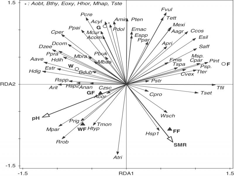
Figure 1:
RDA ordination diagram of nematode communities and Soil pH and Soil Microbial Respiration (Resp) as constrained variables in different ecosystems: forest F; forest with F. japonica FF; grassland G; grassland with F. japonica GF; wetland W; wetland with F. japonica WF with 53.5% 500 explained variance (eigenvalues of axis: 0.35; 0.19; pseudo F = 1.7; P = 0.01). For abbreviation of species see Table 2. Empty circles: biotopes without F. japonica, full triangles: biotopes with F. japonica.
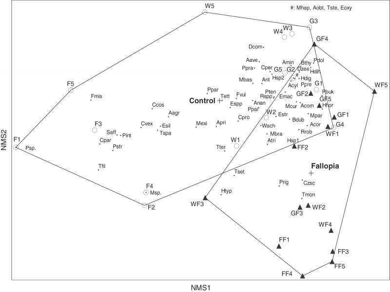
Figure 2:
NMS analysis of samples characterized by nematode species abundance, the grouping factor is presence/absence of F. japonica. Plus signs stand for centroids of two groups, lines around groups connect the outer points of a group. Empty circles represent soil samples from Control: forest F1 to F5, grassland G1 to G5, and wetland W1 to W5. Full triangles represent soil samples with invaded plan F. japonica: forest with F. japonica FF1 to FF5; grassland with F. japonica GF1 to GF5; wetland with F. japonica WF1 to WF5. For abbreviation of species see Table 2. Variance explained by axis 1 and 2 is 48 and 28%, respectively.