Comparative study of Kalman filter-based target motion analysis by incorporating Doppler frequency measurements

With the miniaturization of technology, small urban and domestic drones and robots are ubiquitous. These self-driving machines are applied in parcel and food delivery (Jang and Kim, 2019), rescue missions (Alexopoulos et al., 2013), surveying, and security (Pham et al., 2015). Drones are flying and navigating through congested urban environments while performing assigned tasks (Li et al., 2019). Although these applications seem different but detecting static and dynamic objects (targets) in surroundings is a key requirement by all. The problem of target location and velocity estimation is commonly known as Target Motion Analysis (TMA) (Jang and Kim, 2019; Jauffret and Pillon, 1989;, Li and Jilkov, 2003), and has different variants based on the collected measurement types. Aerospace industry has strict weight and size limits for any additional sensor that can be placed on the drone. Sensors required for avoiding collisions has to be simple, low-powered, and rugged (Li et al., 2019). Moreover, successful utilization of such collision avoidance systems lies in its miniaturization and smooth integration (Jin et al., 2020). Currently, a lot of focus is put on collision avoidance using cameras (Quan et al., 2020). However, cameras are sensitive to environmental conditions (rain, fog, dust), are computationally expensive, and require high operating power (Lee et al., 2016; Ciaparrone et al., 2020).

Radars, on the other hand, are quite robust to light and environmental conditions. Doppler radars are simplest types of radars, that are cheap, require less power, and are computationally inexpensive (Al-Hourani et al., 2018). They capture the Doppler frequency shift in the transmitted and reflected radio signals to obtain the target’s relative velocity. However, these radars cannot provide the target’s range. Simultaneous estimation of range and velocity is done by using more sophisticated and costly radars, such as Frequency or Pulse Modulated Continuous Waveform radars. However, these radars suffer from other issues like waveform design, power consumption, etc., Al-Hourani et al. (2018). In this work, we address the problem of estimating a target’s range and velocity by incorporating Doppler frequency measurements from a simple continuous wave Doppler radar.

Bearings-only target motion analysis (BOTMA) is a well-studied problem (Jauffret and Pillon, 1989; Nardone and Aidala, 1981; Jauffret and Pérez, 2018; Arulampalam et al., 2020). The convergence and observability conditions associated with bearings-only measurements are well-known (Arulampalam et al., 2020; Do˘gançay, 2015). However, contrary to the simplicity of the Doppler radars, Doppler frequency-only target tracking (FOTMA) (Jauffret and Pérez, 2018) is a complex problem, where observability of target’s range and velocity is not fully understood. Several intrinsic research issues in FOTMA must be addressed before this technology can be used as a position and velocity estimator on drones, robots, and other machines.

The goal of this paper is to estimate target’s motion using Doppler measurements from a continuous wave Doppler radar. We discuss the necessary and sufficient conditions required for convergence of target’s range estimation to a unique tracking solution. The main contributions of this paper are: (i) to use the simple Continuous Wave Doppler radars to obtain range and absolute velocity information of targets, (ii) designing simple motion patterns feasible for drones and robots that guarantees the convergence of recursive Kalman filter-based methods to a unique solution, (iii) analyzing and comparing the performance of non-linear Kalman filter based methods for our problem settings. Unlike bearings-only solutions, which takes tens of seconds (Arulampalam et al., 2020; Jauffret et al., 2017), our approach of incorporating Doppler measurements converges within fraction of a second. Performance of the trackers is compared on the basis of Root Mean Square Error (RMSE), number of divergent tracks in 1,000 Monte-Carlos (MC) runs, and time required to converge to the final solution.

The paper is organized as follows: in the second section, we review the associated literature. In the third section, we design the problem as state-space model, discuss observability conditions, and its requirements. We also present the non-linear Kalman filter methods required to update the model as new measurements arrive and for convergence to a unique localization solution. We design and experiment with different simulation scenarios to compare the localization performance of three Kalman approximate filter under different measurement sets. Conclusions and discussion follow in the last section.

Literature review

Passive target tracking and localization using radars is a widely studied estimation problem, commonly known as Target Motion Analysis (TMA) (Jauffret and Pillon, 1989; Nardone and Aidala, 1981; Jauffret and Pérez, 2018; Arulampalam et al., 1981; Kumar et al., 2021). For example, in avionics for tracking planes and missiles (Hügler et al., 2018; Walker et al., 2019), in robotics and machine vision for tracking people (Piriyajitakonkij et al., 2020) and objects of interest (Skaria et al., 2020), in underwater environments for tracking submarines and sea fauna (Luo et al., 2018), etc. With advancements in machine learning and availability of powerful computers, researchers have approached this problem using deep learning methods (Liu et al., 2020; Skaria et al., 2019) as well. However, in case of drones, we have strict weight and power limitations, that restricts the use the computationally expensive deep learning methods or computer vision-based solutions in current problem’s framework.

A main requirement of the tracking algorithm is to guarantee the uniqueness of the solution (Arulampalam et al., 2020). Traditional radar-based target tracking methods consider a single observer that monitors the movements of a target by taking measurements and subsequently estimating its position and velocity. Depending upon the nature of target’s dynamics and resulting measurements, the system could be linear or non-linear (Li and Jilkov, 2003). A given dynamic system is considered observable (Jauffret et al., 2017; Pillon et al., 2016) if its state can be uniquely determined from its model, inputs, and outputs. In practice, precise knowledge of such conditions is required under which a unique solution could be guaranteed.

For analysis with bearings-only measurements, one of the widely used methods is to transform non-linear measurements into a linear form. Then we can use theorems from linear systems’ theory for observability analysis (Nardone and Aidala, 1981; Hammel and Aidala, 1985). However, this approach led to complicated non-linear differential equations that require tedious mathematics to obtain a solution. Moreover, results obtained from this technique are also quite cumbersome to be interpreted for real life. An elegant approach proposed by (Fogel and Gavish, 1998; Becker, 1993) avoids analyzing the observability matrix altogether. It develops the uniqueness criterion for two-dimensional first-order (Payne, 1989), three-dimensional second-order (Jauffret and Pillon, 1989) and general three-dimensional Nth order target dynamics case by using simple linear system theory approach and geometric analysis.

When only frequency measurements are available, to the best of our knowledge, no one has yet been able to recast them into linear form (Becker, 1993). For a constant velocity model and a specific scenario (Shensa, 1981), derived observability conditions for Doppler frequency-only tracking. Although it provides useful geometrical insights when the solution is unique, up to a rotation and reflection in the observer’s coordinate system, results, and discussions are only limited to a fixed velocity target.

For combined set of bearings and frequency measurements, non-linear equations can be recast into linear form, leading to necessary and sufficient observability conditions for two-dimensional first-order dynamics case (Passerieux et al., 1988) and Nth-order dynamics case (Fogel and Gavish, 1993; Becker, 1993). Researchers (Jauffret and Pillon, 1989; Jauffret and Pillon, 1996) analyzed the observability issue of BFTMA for continuous-time and in (Jauffret and Pérez, 2018); for discrete time. They developed the observability conditions by converting state estimation equations into a pseudo linear form. However, this introduced an inherent bias in the model, which they subsequently tried to remove by formulating an unbiased estimator.

Given the non-linearity and Nth order dynamics nature of our problem, we adopt the observability criterion developed in (Becker, 1993), where no restriction is imposed on observer and target’s motion. Becker (1993) first determines the set of all the trajectories compatible with the given measurements. Next necessary and sufficient observability conditions are obtained that reduces the set of possible trajectories to a unique tracking solution. The observability conditions, thus, obtained lend themselves to straightforward physical interpretations. In the next section, we design simulation scenarios, where we manoeuvre the observer according to these observability conditions and measure the estimator’s performance.

Target motion analysis

Potential targets in an indoor environment include walls, furniture, and people etc. We aim to localize and track all such indoor targets surrounding the observer. However, to keep things simple and establish a base framework, we first assume the case of a single observer and a target. We also assume that the observer can focus on the target at all times – getting its bearings and Doppler frequency measurements. To this end, consider the observer target geometry shown in Fig. 1.

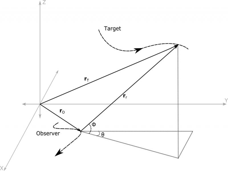
Figure 1:

An observer moving along trajectory${\overline{r}}_O(t)$ takes the bearing and frequency measurements of a target T moving along a trajectory ${\overline{r}}_T(t)$ and emitting a signal of frequency fo. We can obtain the following relation from the geometry in Fig. 1.(1)

We have simulated continuous wave Doppler radar operating at 24 GHz, with one transmitting and one receiving array. The receiver produces the I and Q components of the beat signal using sampling frequency of fs = 8000 Hz. Moreover, we simulated a narrow beam with width and elevation of ${10}^0$. We consider three measurement sets, namely, bearings-only, frequency-only, and bearing-frequency measurements together. The bearings $(\theta )$ and Doppler frequency $(f_d)$ measurements satisfy following relationships (Skolnik, 2001),(2)(3)

• r-x${\overline{r}}_x$ and ${\overline{r}}_y$ are X and Y components of $\overline{r}(t)$,

• ${\overline{V}}_R$ is the radial velocity vector,

• $\lambda$ is signal’s wavelength, and

• $f_d$ is Doppler frequency.

CASE-1: manoeuvring observer

In this scenario, we consider a dynamic observer that moves around in a $(5\times 5){\mathrm{m}}^2$ room and tries to estimate the range of a point-like target located at $x=5\mathrm{m}$ and $y=5\mathrm{m}$ using bearing and frequency measurements. The target-observer geometry for this scenario is shown in Fig. 2.

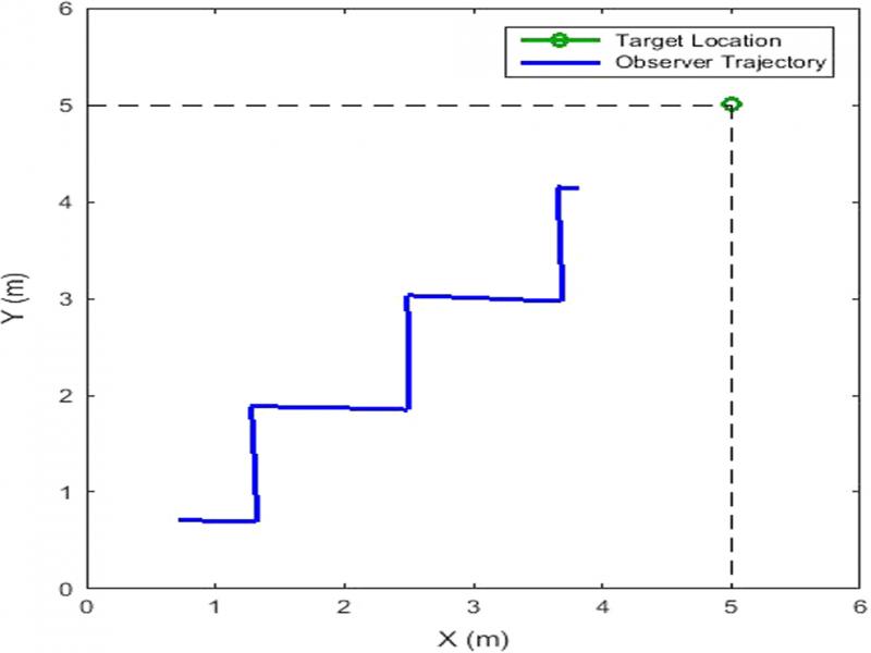
Figure 2:

The observer starts at coordinates $x=1\mathrm{m},$$y=1\mathrm{m}$, y = 1m moves with velocity 10 km/h (2.8 m/s) and exhibits 90° maneuvers from time to time (Arulampalam, 2000), as follows,

• From 90° to 0° at time t = (20 + 200k) Tsec, k = [0, 1, 2, …]$t=(20+{200}^k)Tsec,k=[0,1,2,\mathrm{\dots }]$

• From 0° to 90° at time t = (100 + 200k) Tsec, k = [0, 1, 2, …]$t=(100+{200}^k)Tsec,k=[0,1,2,\mathrm{\dots }]$

where T is sampling time.

Let $X_T[k]$ and $X_O[k]$ denote target’s and observer’s state at time instant k. Position and velocity components in $X_T[k]$ and $X_O[k]$ are arranged as,(4)

(4)

$$\begin{array}{}\text{(4)}& X_O[k]=[\begin{array}{l}\mathrm{xposition}\hfill \\ \mathrm{xvelocity}\hfill \\ \mathrm{yposition}\hfill \\ \mathrm{yvelocity}\hfill \end{array}]=[\begin{array}{l}x\hfill \\ V_x\hfill \\ y\hfill \\ V_y\hfill \end{array}].\end{array}$$

For constant velocity scenario, observer’s dynamics can be modeled as a Constant Velocity Model (Li and Jilkov, 2003; Bar-Shalom and Li, 2001). It assumes that the target moves with constant velocity where small perturbations are modeled as independent acceleration noise. It is given as,(5)

(5)

$$\begin{array}{}\text{(5)}& X_O[k+1]=F{X}_O[k]+U[k]+Gv[k],\end{array}$$

where F is state transition matrix defined as,(6)

(6)

$$\begin{array}{}\text{(6)}& F=[\begin{array}{cccc}1& T& 0& 0\\ 0& 1& 0& 0\\ 0& 0& 1& T\\ 0& 0& 0& 1\end{array}].\end{array}$$

U[k] is the deterministic input vector, which accounts for the effect of observer accelerations. U[k] is deterministic since we assume that we have the knowledge of observer state $X_O$ at every instant of time. The Gain matrix G is(7)

(7)

$$\begin{array}{}\text{(7)}& G=[\begin{array}{cc}\frac{T^2}{2}& 0\\ T& 0\\ 0& \frac{T^2}{2}\\ 0& T\end{array}],\end{array}$$

v(k) is zero-mean white Gaussian noise process with variance ${\sigma }_v$. The covariance of noise process multiplied by gain G is given as,(8)(9)(10)

(8)

$$\begin{array}{}\text{(8)}& Q=E[Gv(k)v(k)G\text{'}],\end{array}$$

(9)

$$\begin{array}{}\text{(9)}& ={\sigma }_v^{2}GG\text{'},\end{array}$$

(10)

$$\begin{array}{}\text{(10)}& ={\sigma }_v^2[\begin{array}{llll}\frac{T^4}{4}\hfill & \frac{T^3}{2}\hfill & 0\hfill & 0\hfill \\ \frac{T^3}{2}\hfill & T^2\hfill & 0\hfill & 0\hfill \\ 0\hfill & 0\hfill & \frac{T^4}{4}\hfill & \frac{T^3}{2}\hfill \\ 0\hfill & 0\hfill & \frac{T^3}{2}\hfill & T^2\hfill \end{array}].\end{array}$$

We can now introduce the relative state vector as,(11)

(11)

$$\begin{array}{}\text{(11)}& X[k]=X_T-X_O\end{array}$$

The corresponding state equation for relative state vector is,(12)

(12)

$$\begin{array}{}\text{(12)}& X[k+1]=FX[k]-U[k]+Gv[k]\end{array}$$

Measurement vector $Z[k]$ is related to state $X[k]$ through non-linear function $h(.)$ as,(13)

(13)

$$\begin{array}{}\text{(13)}& Z[k]=h(X[k])+w(k),\end{array}$$

where $w(k)$ is 0 mean white Gaussian observation noise with variance ${\sigma }_w$σW .h(.) $h(.)$ is a non-linear function of the state, whose value depends on the measurements being considered.

• For bearings only measurements, angle $\theta$ is measured counter-clockwise from positive X-axis.(14)

  (14)

  $$\begin{array}{}\text{(14)}& h(x[k])=\theta ={\tan }^{-1}(\frac{R_y(t)}{R_x(t)}).\end{array}$$

• For Doppler or relative velocity $(V_R)$ only measurements,(15)

  (15)

  $$\begin{array}{}\text{(15)}& h(x[k])={\overline{V}}_R=\frac{R_x{\overline{V}}_x+R_y{\overline{V}}_y}{\sqrt{R_x^2+R_y^2}}.\end{array}$$

• For bearings and velocity $(V_R)$ measurements together,

(16)

$$\begin{array}{}\text{(16)}& h(x[k])={[\theta ,V_R]}^{{\rm T}},\end{array}$$

where superscript ${\rm T}$ means vector transpose.

Covariance matrix $R_{ww}$ of measurement noise is given by σ2wI, where I is the identity matrix whose size depends upon $h(x[k])$ and ${\sigma }_w$ is standard deviation of the measurement noise.

According to the observability criterion developed in Becker (1993), depending upon the measurements, target’s state is observable when following conditions are met:

• Bearings-only Measurements: LOS angle must not remain constant.

• Doppler-only measurements: LOS angle must not be constant and observer’s dynamics must be at least two degrees higher than target’s motion.

• Bearing and Doppler Measurements: LOS angle must not remain constant

The optimal Bayesian solution to this problem requires computing the posterior density $p(X[k]|Z[k])$. However, this is not possible because measurements’ Equation (13) is non-linear. Therefore, we have to suffice for suboptimal solutions and use the methods developed for non-linear systems. Extended Kalman Filter (EKF) (Kalman and Bucy, 1961; Ristic et al., 2004) has been everybody’s go-to option for non-linear systems. It works by linearizing the non-linear state space equations using first-order truncation of Taylor series. However, this approximation is only useful if second and higher order derivatives are effectively 0 (Julier and Uhlmann, 2004). Otherwise resulting statistics which are linearly calculated are inaccurate. Another major drawback with EKF is that during linearization process, it fails to take into account that X is a random variable. It ignores the probabilistic spread of X modeled as covariance $P_{XX}$, and linearizes it around a single point. This introduces large errors in later stages and affects the consistency of the filter. Posterior mean and covariance calculated do not represent the actual scenario and, more than often, filter ends up diverging.

To overcome these and other shortcomings of EKF, researchers have developed numerous approximations of Kalman filter for non-linear systems. These algorithms are closely related as how they handle multi-modal integrals in Bayes formula. Instead of linearizing the non-linear equations, these algorithms depend upon deterministic sampling methods for the propagation of Gaussian random variables through non-linear systems. Unscented Kalman Filter (UKF) (Julier and Uhlmann, 2004) uses scaled unscented transformation to compute the points that can capture the current statistics of Gaussian Random Variables. Then it uses these points through the non-linear systems, thus avoiding the requirement of Taylor Series truncation. In more recent developments, Cubature Kalman Filter (CKF) (Arasaratnam and Haykin, 2009) was introduced as a more robust and stable version to handle the multi-model Bayes integrals. Underlying idea is same as that of Unscented Kalman Filter; however, it uses Cubature rules to handle the integrals.

In this work, we implemented and compared the performance of Extended Kalman Filter (EKF), Unscented Kalman Filter (UKF), and Cubature Kalman Filter (CKF). Performance comparisons are based on a set of 1,000 Monte-Carlo (MC) runs (Ristic et al., 2004). The performance metrics used in our analysis are Root-Mean-Square (RMS) error and number of divergent tracks in 1000 MC runs. RMSE is calculated as follows,

(17)

$$\begin{array}{}\text{(17)}& \mathrm{RMSE}=\sqrt{\frac{({\sum }_{i=1}^N{(X_i-{\hat{X}}_i)}^2)}{N}}.\end{array}$$

A track is classified as divergent if at any time, the estimated position error of the target exceeds a preset threshold. This threshold is set depending upon the geometry of the problem at hand, which in this case is set at 20 m. RMS position error is only computed for non-divergent tracks. Considering the geometry of our scenario and constraints of observer and target dynamics, all filters are initialized with an initial range of 5 m. Standard deviations of range and velocity are chosen to be ${\sigma }_r=3\mathrm{m}$ and ${\sigma }_v=1.673{\mathrm{m}/\mathrm{s}}^2$ . Standard deviation for process noise is ${\sigma }_v=0.5{\mathrm{m}/\mathrm{s}}^2$, whereas, for bearing and Doppler measurements it is chosen to be ${\sigma }_{\theta }=1^{\mathrm{o}}$, and ${\sigma }_{V_r}=0.5\mathrm{m}/\mathrm{s}$, respectively.

Results and discussions

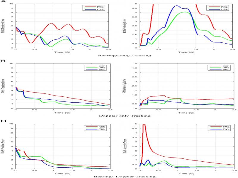
Fig. 3 shows the tracking results for the three non-linear target trackers, namely, bearings-only, Doppler frequency-only, and bearing-Doppler trackers. Each run simulates 2.5 s of the scenario, allowing the observer to finish about six maneuvers. Table 1 shows the position and velocity RMSE for the three filters.

Table 1.

Comparing performance of non-linear Kalman Filters for abruptly manoeuvring observers.

Figure 3:

For bearings-only case, we can see in Fig. 2 that RMSE decreases with each manoeuvre. After 2.5 s and six maneuvers total RMSE dropped to about 1.14 m for EKF, to 0.11 for UKF, and to 0.24 CKF. This convergence to the unique final solution means that tracker is successfully meeting the observability conditions.

For Doppler frequency-only measurements, RMS position error also decreased continuously with each manoeuvre, as shown in Fig. 2. After 2.5 s, RMSE for EKF dropped to about 0.94 m whereas, for UKF and CKF it dropped to 0.6 m. In this case, as well, both UKF and CKF performed better than EKF.

When both the bearings and the Doppler frequency measurements are used, target trackers converged much faster, as shown in Fig. 2. RMSE dropped to 1 m with three maneuvers in the first second. This error decreased even further, reaching 0.5 in 2.5 s for EKF and below 0.01 m for both UKF and CKF, as shown in Fig. 2.

Out of 1,000 MC runs, EKF diverged about 200 times, whereas UKF and CKF diverged about 4 and 3 times, respectively.

The results showed that localization gets better with each 90° manoeuvre. However, such abrupt maneuvers are unrealistic in real life where observer’s dynamics are constrained and limited. For example, consider the case of a radar fitted on top of a drone. In this case, it will not be practical for drone to do these sudden 90° maneuvers. Next, we discuss the observer’s maneuvers that are practical and still meet observability constraints.

CASE-2: circular moving observer

The problem at hand is that we want to find a practical motion pattern for the observer, which meets the observability requirements – giving us a unique solution to the tracking problem (Becker, 1993). The main conditions are that the line-of-sight (LOS) angle must not remain constant, and the observer’s motion must be of two degrees higher than the target’s movement. Although abrupt 90° maneuvers are not practical for drones or other such machines, it is relatively easy for them to move in a circular pattern. When the observer moves in a circular pattern, then it meets both observability requirements. First, the line of sight angle keeps changing, and secondly, because of the observer’s circular motion, the relative motion dynamics has infinite derivatives.

In this second simulation scenario, we test and verify that a circular moving observer meets the observability conditions. The observer now moves on a circular trajectory while taking the target measurements. Target is again assumed to be stationary at coordinates (5,5). Target-Observer track geometry in this case is shown in Fig. 4.

Figure 4:

In this case, observer’s motion is better modeled as coordinated turn model (Li and Jilkov, 2003; Laneuville, 2013; Roth et al., 2014). We assume that observer moves with a known constant speed and turn rate $(\omega )$. In case of known turn rate, state vector remains the same as in (4). The state transition matrix in Equation (5) now becomes,

(18)

$$\begin{array}{}\text{(18)}& F=[\begin{array}{cccc}1& \frac{\sin (\omega T)}{\omega }& 0& -\frac{1-cos(\omega T)}{\omega }\\ 0& \cos (\omega T)& 0& -\sin (\omega T)\\ 0& \frac{1-cos(\omega T)}{\omega }& 1& \frac{\sin (\omega T)}{\omega }\\ 0& \sin (\omega T)& 0& \cos (\omega T)\end{array}],\end{array}$$

(18)and covariance matrix $Q$ (8) now becomes,

(19)

$$\begin{array}{}\text{(19)}& Q=[\begin{array}{llll}\frac{2(\omega T-\sin (\omega T))}{{\omega }^3}\hfill & \frac{1-\cos (\omega T)}{{\omega }^2}\hfill & 0\hfill & \frac{\omega T-\sin (\omega T)}{{\omega }^2}\hfill \\ \frac{1-\cos (\omega T)}{{\omega }^2}\hfill & T\hfill & -\frac{\omega T-\sin (\omega T)}{{\omega }^2}\hfill & 0\hfill \\ 0\hfill & -\frac{\omega T-\sin (\omega T)}{{\omega }^2}\hfill & \frac{2(\omega T-\sin (\omega T))}{{\omega }^3}\hfill & \frac{1-\cos (\omega T)}{{\omega }^2}\hfill \\ \frac{\omega T-\sin (\omega T)}{{\omega }^2}\hfill & 0\hfill & \frac{1-\cos (\omega T)}{{\omega }^2}\hfill & T\hfill \end{array}].\end{array}$$

Remaining algorithm and simulations settings remain the same as in the previous section.

Results and discussions

Fig. 5 illustrates the tracking results obtained by averaging 1,000 MC runs for the three trackers considered. Main thing to note here is that with observer’s circular movement, trackers converged within fraction of a second.

Figure 5:

For bearings-only measurements, EKF showed poor RMSE of 1.5–2 m. UKF converged to 0.4 m RMSE within 0.2 s and then stayed at this value. CKF also showed good performance localizing target’s position within 0.5 cm. However, unlike UKF tracker, it converged to this value gradually over time. For Doppler frequency-only measurements, EKF diverged about 80% and reaching an RMSE of 2.4–2.9 m. Both UKF and CKF converged to 0.5 m RMSE in 0.2 s. Excellent results were obtained with bearing-frequency measurements. UKF and CKF successfully localized the target to 0.1 m accuracy and were also able to measure velocity with high accuracy and low RMSE of 0.2–0.3 m/s. Table 2 shows the result of target tracking with circular moving observer.

Table 2.

Comparing performance of non-linear Kalman filters for circular moving observers.

	Position RMSE (m)			Velocity RMSE (m/s)
Measurements set	EKF	UKF	CKF	EKF	UKF	CKF
Bearings-only	1.14	0.11	0.24	1.25	0.83	0.45
Doppler frequency-only	0.94	0.63	0.61	1.23	0.38	0.49
Bearings-frequency measurements	0.52	0.01	0.01	0.91	0.62	0.26

Out of 1,000 MC runs, EKF diverged about 213 times, whereas UKF and CKF did not diverge at all.

Unlike linear filters, the non-linear ones are quite sensitive to initial conditions. In our case, filters with Doppler-only measurements are quite sensitive to the initial velocity values. However, filters based on bearings-frequency measurements together performed much better even with improper initialization.

Conclusions

Finding the relative position of objects in urban and indoor environments is a key challenge for tiny observers, e.g., drones and robots. In this research, we have introduced the idea of analyzing a target’s motion by incorporating Doppler frequency measurements. Observability analysis showed that with frequency-only measurements line-of-sight angle must change and that the observer’s motion dynamics must be at least two degrees higher than target’s motion. However, with bearing-frequency measurements together, the only observability requirement is that line-of-sight angle between observer and target does not remain constant. On the basis of these observations, we designed and compared the performance of three non-linear Kalman approximate filters. Performance was measured in terms of root mean squared position error, velocity error and total number of divergent track in 1,000 MC runs. The results showed that when observability conditions are met then we are able to track targets with accuracy using frequency-only targets. Moreover, we also devised the motion patterns that an observer can follow to meet the observability conditions and localize targets in the surroundings. We also presented the idea of circular motion for drones and machines to localize the targets. The results showed that with this strategy an observer can successfully estimate the position of targets within fraction of a second. Bearings-only target trackers, comparatively require tens of seconds to converge (Jauffret and Pérez, 2018; Arulampalam et al., 2020; Pillon et al., 2016). Moreover, our approach is computationally much more efficient then latest deep learning based methods, making it an ideal candidate for collision avoidance using continuous wave Doppler radars on small drones and robots. Among the three trackers, UKF performed better than CKF and EKF. Best results were achieved using bearing-frequency measurements together with UKF.

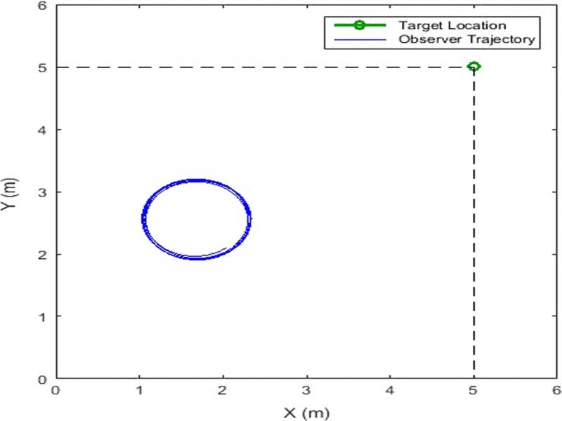
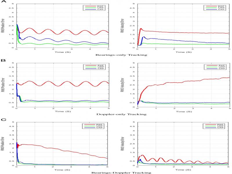
	Position RMSE (m)			Velocity RMSE (m/s)
Measurements set	EKF	UKF	CKF	EKF	UKF	CKF
Bearings-only	2.2	0.4	0.5	1.6	0.4	0.5
Doppler frequency-only	2.7	0.5	0.7	3.3	0.3	0.5
Bearings-frequency measurements	0.7	0.1	0.1	0.4	0.2	0.2