A new HGA-FLVQ model for Mycobacterium Tuberculosis detection

Methods

Main points relating to the development of model are described in this section. First, the below equation based on (Dahlan, 2010) calculating the sample size for this research is explained. Second, the developed block model and tasks of each block are elaborated. Third, various processes of the overall development of model are discussed from the beginning to the end. The developed model in this research is presented in Figure 1.

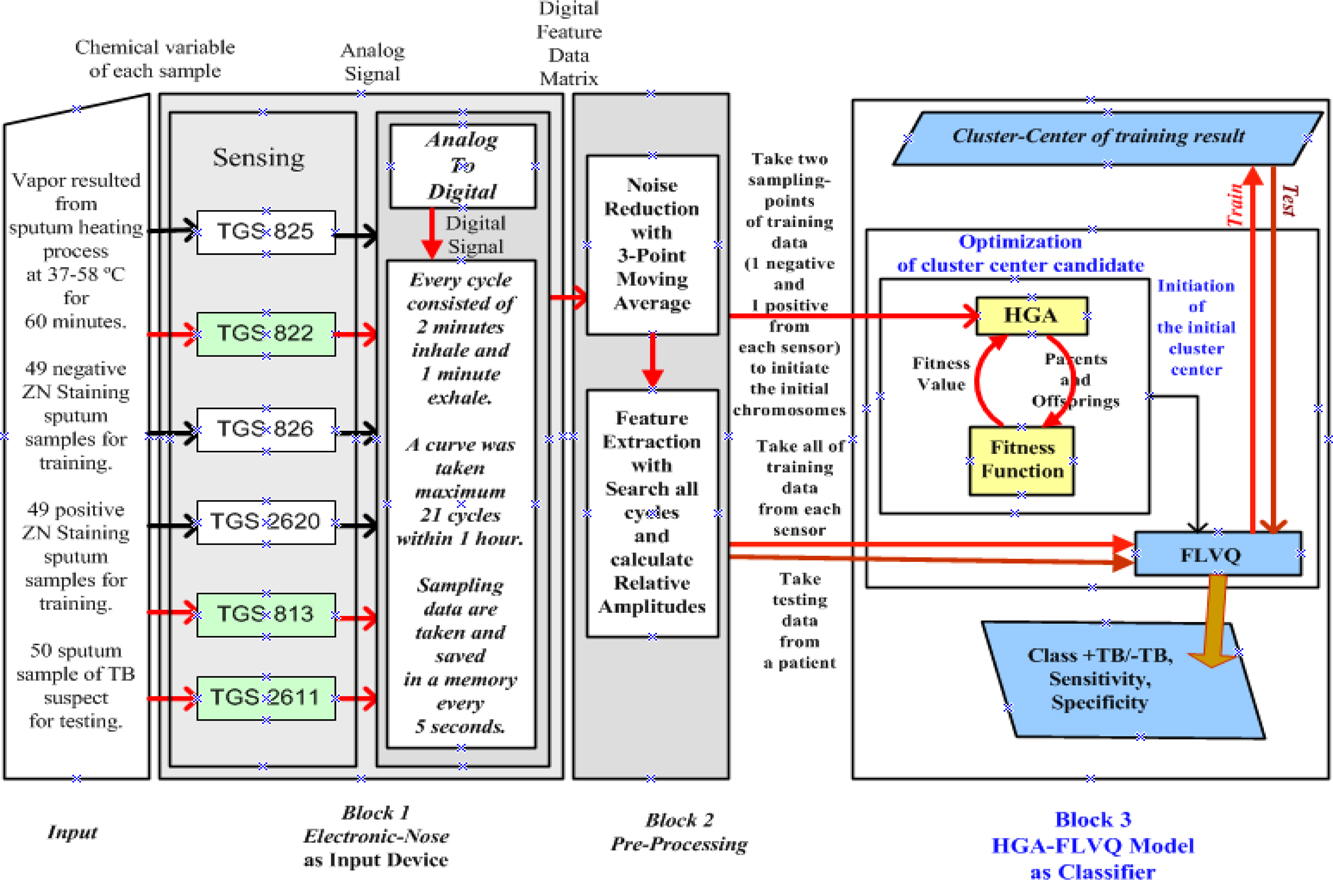
Figure 1

In this research, the sample size was calculated based on (Dahlan, 2010) the following equation:

Here, n denotes the research sample size, Sen is the expected sensitivity of the model of which the diagnostic value was tested, d is expected research precision, α is the accepted error rate to determine the deviation standard (Z_α), and P is the prevalence of TB disease (the proportion of positive-TB patients among the TB suspects).

The following is the implementation of Equation (1) in this research. The error rate of type 1 (one direction) that is still accepted (α) equals 5%. The deviation standard (Z_α) is 1.96. The expected sensitivity is 90%. The expected research precision (d) is 10%. The TB prevalence (P), referring to the proportion of positive-TB patients after an assessment of overall TB suspects in 2015 who received medical treatments from Prof. Dr. Barmawi Hisyam, Sp.P.D.-KP, equals 70%. Hence, the research sample size is as follows:

It is rounded up to 50 TB suspects.

After receiving Ethics Committee Approval from Medical and Health Research Ethics Committee (MHREC), Faculty of Medicine, Universitas Gadjah Mada, with Ref number: KE/FK/71/EC/2016, primary data retrieval at this research could be started in TB laboratory, Faculty of Medicine, Universitas Gadjah Mada.

The e-nose device employed in this research consisted of six sensors, namely, TGS822, TGS813, TGS2611, TGS825, TGS826, and TGS2620. However, primary data (training data and testing data) of this research were only obtained from three sensor response curves. The sensors used in this research were TGS822, TGS813, and TGS2611, as the other sensors were not adequately responsive and were selective to significantly distinguish the characteristics of patients (relative amplitudes) of the positive ZN staining and the negative ZN staining, using direct eye observation. Each period of the electronic-nose response curve of the three sensors was sampled every 5 sec.

There were three categories of samples, namely 49 negative ZN staining subjects’ sputum samples, 49 positive ZN staining patients’ sputum samples, and 50 sputum samples of TB-suspected patients who received medical treatments at Public Health Centers in Yogyakarta and A RESPIRA Pulmonary Hospital of Yogyakarta Province between February 25 and May 8, 2016. An inclusion criterion of negative-TB samples was when a patient was diagnosed as a TB suspect by the doctor, but the patient was declared contrary by laboratory examination using the ZN staining sputum method. Meanwhile, the inclusion criterion of positive-TB samples was when a positively suspected TB patient was declared positive-TB using ZN staining sputum method. Exclusion criteria from positive-TB samples were +HIV subject and positive-TB in extrapulmonary.

Sensing and sampling processes shown at the first block of Figure 1 are elaborated. The sputum samples of this research were obtained three times. First time, on the first day, the suspected patient’s sputum was obtained when the TB-suspected patient visited the Public Health Center for the first time, and then the TB-suspected patient brought a sputum pot containing the sample on the second day, early in the morning. The second sample was the sputum saved at home, soon after the TB-suspected patient woke up in the early morning on the second day. On that day, the TB-suspected patient brought the sample and handed it over in the sputum pot to the medical officer in the Public Health Center. Third, the sputum sample was accepted again in Public Health Center on the second day, when the TB-suspected patient gave the morning sputum sample. In a biosafety cabinet, the three sputum samples were combined to meet the minimum volume requirement so that evaporation and sensing processes could be carried out. The sputum evaporation of a sample was performed by warming it up at the temperature between 38 and 58°C for 60 min in the electronic-nose sample room. The sensors of electronic-nose devise during the process used VOC as the biomarker to detect the presence of MTB. Then, the sensors calculated the rate of VOC and converted the chemistry magnitude to electrical magnitude (analog signal). After that, an interface application in the electronic-nose device transformed the analog signal of its sensor to a digital signal. The digital signal was presented in the form of response curve from each sensor with its maximum length of 20 cycles. Subsequently, each cycle of the response curve from the electronic-nose device was read or sampled every 5 sec to obtain digital data.

At the second block of Figure 1, the processes consist of two types of pre-processing, namely, noise reduction and feature extraction. Considering that the response curve of the electronic-nose came out from the first block still contained noises, a noise reduction method became essential to apply. The noises could be reduced using a filter as can be seen in Equation (4), and its results were saved in a memory.

Generally, a finite impulse response (FIR) filter as in Smith (1999) for the case of N-Points is shown in the following equation:

Equation (2) can be written as in Kusumoputro et al. (1999) as:

The second process of the second block (pre-processing) in Figure 1 is feature extraction (the feature of positive-TB and feature of negative-TB) from each curve of the electronic-nose response. The feature extraction could be done after the noises significantly decrease. If marker events in this research could be recognized in each curve of the electronic-nose response, the feature extraction in this research (as pre-processing) could be performed through searching peaks and troughs as landmarks or features (James, 2007). These searching cycles were used to obtain relative amplitudes (Ar) from each cycle in the electronic-nose response curve. Ar became the features and primary data in this research. Response curves of the three sensors of electronic nose were not involved in the processes of feature extraction as an observation unit, because each sensor had the unique response when sensing was performed so that the calculation of Ar was performed for each response curve individually. The response signal of each sensor illustrated amplitude in time function forming a pattern (Kusumoputro et al., 2002). In this research, features of the sensor response signal were extracted using the following equation, as shown in a study Hardoyono et al. (2015) and Figure 2:

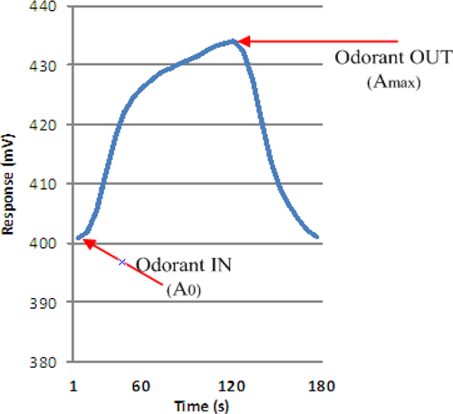
Figure 2

At the third block, there are three processes in the hybrid genetic algorithm-fuzzy learning vector quantization (HGA-FLVQ) model as displayed in Figure 1. In the first process, HGA read and normalized data from the pre-processing result (all of the training data) of each sensor’s output in the pre-processing block.

The second process was the process of assisting initialization of FLVQ artificial neural network so that FLVQ could have an optimal initial cluster center. This process executed HGA operators in the HGA-FLVQ model. Then, the HGA method took the first two Ars of each class (positive-TB and negative-TB) from the training data to become two parents. After that the two parents were processed by simulated-annealing recombination (SAR) function and simulated-annealing mutation (SAM) function in HGA (Adler, 1993). A crossover operator in SAR function and a mutation operator in SAM function were implemented repeatedly. Every time HGA produced two offsprings, the values of fitness from these offsprings were also calculated to determine whether those two offsprings were accepted in the new generation population. If the offspring fitness value was better than the parent fitness value, then that offspring was used to replace its parent. However, if not, then it was ignored, and the Ar cluster center of the final generation of this HGA was used for initialization of FLVQ artificial neural network.

The third process of HGA-FLVQ model was model training performed by FLVQ artificial neural network. In this research, this model training was carried out repeatedly using the sputum samples of a group of 98 patients consisting of 49 positive ZN staining patients, 40 negative ZN staining patients, and 9 healthy volunteers who had never been diagnosed with TB by a doctor. The training process using the FLVQ method can be elaborated as follows. Initialization of the initial cluster center was performed by taking HGA output of each sensor. Then, some variables were calculated repeatedly until the desired minimum error was obtained. Those variables were the weighting exponent (also referred to as fuzziness parameter), learning-rate factor (alpha), learning-rate, new cluster center, and error. Afterward, the last cluster center of each sensor data of each class was saved in a memory as a result of training.

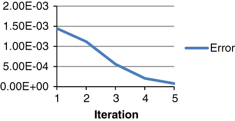
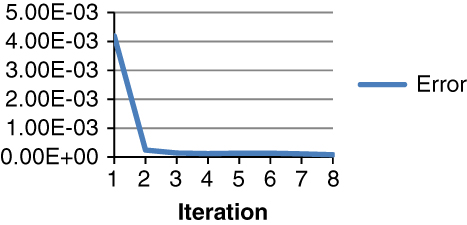
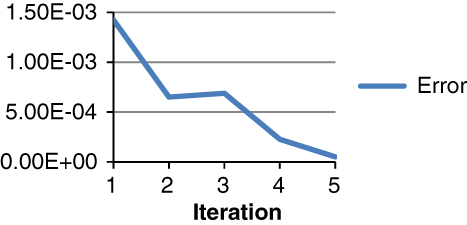
This section also elaborates the result of HGA-FLVQ model training as displayed in Table 2. The process of this HGA-FLVQ model training from TGS813, TGS822, and TGS2611 sensors lasted for 5 to 8 iterations since the error decreased below 0.0001. The error reduction process occurred on each iteration as shown in Figures 3,4, 5.

Table 2

Results of HGA-FLVQ model training.

Figure 3

Figure 4

Figure 5

Training processes using LVQ and FLVQ methods as comparator methods are elaborated in the following parts. Learning vector quantization (LVQ) aiming at classifying training data of n vectors into c clusters is one of the learning methods in the artificial neural network (Kusumadewi dan and Hartati, 2010). LVQ is a simple way algorithm applied to the multiclass problem and the complexity of LVQ can be controlled during training phase according to specific needs (Elly et al., 2013).

In the training process of the LVQ method, the weight vector from the input unit to the output unit was referred to as a reference vector (codebook) for the class that the output unit represents. The output unit was positioned by adjusting the weight through supervised training. In this case, the target (a set of patterns with known classification) was provided along with the initial distribution of the reference vector. The training using the LVQ method classified the input vector into the same class as the output unit that has a weight vector closest to the input vector (Widodo, 2005).

In this research, the result of the training using LVQ method is presented in Table 3. The stability of weight value appeared after the 10th iteration, either for the negative or positive class used the training data of each sensor. It could be seen that the weight value either of the negative or positive class for the last iterations was stable at a certain number.

Table 3

Results of weight calculation and revision of LVQ training.

TGS813 Sensor data
Iteration	Fuzziness parameter	Learning rate		Cluster center		Error
1	1.100590	0.000987	0.001400	0.108494	0.024354	0.0014483775
2	1.101180	0.001541	0.000924	0.140709	0.033404	0.00111976
3	1.101770	0.002089	0.000798	0.163612	0.039210	5.5822276E-4
4	1.102360	0.002508	0.000750	0.177564	0.042487	2.0541892E-4
5	1.102950	0.002808	0.000727	0.186139	0.044436	7.73241E-5
TGS822 Sensor data
1	1.100590	0.001144	0.001169	0.093718	0.212932	0.004191581
2	1.101180	0.001008	0.001355	0.097408	0.228077	2.4299692E-4
3	1.101770	0.000919	0.001562	0.102777	0.238711	1.41901E-4
4	1.102360	0.000857	0.001782	0.107080	0.248823	1.207616E-4
5	1.102950	0.000807	0.002042	0.110949	0.259704	1.3338469E-4
6	1.103540	0.000769	0.002332	0.114258	0.270786	1.3375138E-4
7	1.104130	0.000742	0.002620	0.116887	0.280968	1.105932E-4
8	1.104720	0.000723	0.002887	0.118887	0.289624	7.890986E-5
TGS2611 Sensor data
1	1.100590	0.000644	0.005906	0.031570	0.029312	0.0014235964
2	1.101180	0.001916	0.000857	0.055587	0.020714	6.50747E-4
3	1.101770	0.002333	0.000767	0.081313	0.015552	6.8849424E-4
4	1.102360	0.003203	0.000704	0.096225	0.017693	2.2693272E-4
5	1.102950	0.003725	0.000683	0.103321	0.018730	5.1426956E-5

On the other hand, the training process using the FLVQ method is elaborated as follows. At first, an initialization of the initial cluster center was performed by taking the first item of relative amplitude of each sensor. Then, the next process calculated some variables repeatedly until the desired minimum error was obtained. The variables used were weighting exponent (also referred to as a fuzziness parameter), learning-rate factors (alpha), learning-rates, new cluster centers, and an error.

Afterward, the last new cluster centers of each sensor data of each class were saved in a memory as the results of training. In this research, the results of training using the FLVQ method can be seen in Table 4. It is shown that the error decreased below 0.0001 before the 10th iteration. Its reduction in error is relatively faster compared to the LVQ method that needs up to the 10th iterations to obtain the stable weight.

Table 4

Results of cluster center revisions of FLVQ training.

	TGS813 Sensor	TGS822 Sensor	TGS2611 Sensor
1st Iteration
The weight of the negative class	−0.051673025	0.26946884	−0.003179715
The weight of the positive class	−0.002036426	0.1985224	0.21423542
2nd Iteration
The weight of the negative class	−0.0356808	0.28372976	−3.8830974E-4
The weight of the positive class	0.028204879	0.14191468	0.16531087
3rd Iteration
The weight of the negative class	−0.0029952978	0.3213401	0.00271485
The weight of the positive class	0.052159406	0.10385808	0.13945574
4th Iteration
The weight of the negative class	0.03716613	0.37145796	0.0097912615
The weight of the positive class	0.062625006	0.088705875	0.1361857
5th Iteration
The weight of the negative class	0.07502196	0.407575	0.017326174
The weight of the positive class	0.06537599	0.080875896	0.12186478
6th Iteration
The weight of the negative class	0.09876694	0.42662817	0.02240251
The weight of the positive class	0.06590489	0.07604013	0.1046309
7th Iteration
The weight of the negative class	0.11628124	0.44089812	0.026141549
The weight of the positive class	0.06780671	0.074578255	0.09289357
8th Iteration
The weight of the negative class	0.12786691	0.44939327	0.02856244
The weight of the positive class	0.06953817	0.07365509	0.08497784
9th Iteration
The weight of the negative class	0.13485843	0.45396066	0.029982805
The weight of the positive class	0.07066574	0.07268719	0.08011716
10th Iteration
The weight of the negative class	0.13828559	0.4564701	0.030701837
The weight of the positive class	0.07150341	0.072542615	0.07794089

The last process in this research was testing the HGA-FLVQ model. The testing process of HGA-FLVQ model consisted of four steps, namely, reading the test data, calculating Euclidean distances to determine the classes of each relative amplitude item, deciding the classes of each suspect patient, and calculating specificity and sensitivity of the model.

The first process was reading the test data. This process read Ar data of every cycle in the electronic-nose response curve resulting from the sensing of a sputum sample of each TB-suspected patient.

The second process was determining the class classification from every Ar data item. In general, if P is denoted as X₁, X₂, … ,X_n and if Q is denoted as Y₁, Y₂, … ,Y_n, then d(P, Q) could be calculated as in Johnson and Winchern, (2011) for each sensor using Equation (6). In this research, P_i is a variable, and P_i is training datum Ar, P_is are data training Ar from a TB-suspected patient. Q1s are the cluster centers of the training data resulting from every sensor sensing sputum sample of negative ZN staining patients. Q2s are the cluster centers of the training data produced from every sensor sensing sputum samples of positive ZN staining patients. Then, the total number of Euclidian distances between one variable P_i and three variables Q1s was compared with the total number of Euclidian distances between one variable P_i and three variables Q2s. Then, the value of variable d1 was calculated as shown in Equation (7), and the value of variable d2 was calculated as shown in Equation (8). Then, d1 was compared with d2 to determine a prediction class at the variable P_i. If d1 was lower than d2, then the prediction class at this Ar was represented with ‘1’ (negative), but if the result was contrary or d2 was lower than d1, then the prediction class at this Ar was represented with ‘2’ (positive). This calculation was performed for all Ar variables:

(6)

$d\left(P,Q\right)=\sqrt{{\left(x_1-y_1\right)}^2+{\left(x_2-y_2\right)}^2+\dots +{\left(x_p-y_p\right)}^2}$

(7)

$\mathrm{d}1=\mathrm{d}11\left({\mathrm{P}}_{\mathrm{i}},\mathrm{Q}11\right)+\mathrm{d}12\left({\mathrm{P}}_i,\mathrm{Q}12\right)+\mathrm{d}13\left({\mathrm{P}}_i,\mathrm{Q}13\right)$

(8)

$\mathrm{d}2=\mathrm{d}21\left(P_i,\mathrm{Q}21\right)+\mathrm{d}22\left(P_i,\mathrm{Q}22\right)+\mathrm{d}23\left(P_i,\mathrm{Q}23\right)$

The third process was deciding the classes of each suspect patient by adding up the quantity of the prediction classes (‘1’ and ‘2’). Then, a level of confidence of a new negative class was calculated through the number of prediction classes ‘1’ divided by the total number of the data Ar of the electronic-nose response curve resulting from the sputum sample of each TB-suspected patient. Following this process was the calculation of the level of confidence of the new positive class, the number of prediction classes ‘2’ divided by the total number of the data Ar of the electronic-nose response curve resulted from the sputum sample of each TB-suspected patient.

If the level of confidence in the new negative class is higher than 50%, then the prediction class for the sample of the TB-suspected patient is negative. On the contrary, if the level of confidence in the new negative class is below 50%, then the prediction class for the sample of the TB-suspected patient is positive. If the level of confidence in the new positive class is higher than 50%, then the prediction class for the sample of the TB-suspected patient is positive. On the other hand, if the level of confidence in the new positive class is below 50%, then the prediction class for the sample of the TB-suspected patient is negative.

The fourth process was calculating specificity and sensitivity of HGA-FLVQ model using comparator methods. Specificity is the number of negatives prediction classes as same as the targets (the target classes of test data), and the number is divided by the quantity of all TB-suspected patients. Then, its result is multiplied by 100%. Sensitivity is the number of positives prediction classes as same as the targets, and the number is divided by the quantity of all TB-suspected patients. Then, its result was multiplied by 100%.

Results and discussion

This section explains the result of HGA-FLVQ model testing and the results of the comparator methods testing (LVQ method and FLVQ method). These models and method testings used data from sensing and sampling result of the electronic-nose response curve on the vapor of 50 TB-suspected patients’ sputum. Table 5 presents the recapitulation of HGA-FLVQ model testing result of a patient. In Table 5, target class having value ‘2’ denotes positive ZN staining, target class having value ‘1’ denotes negative ZN Staining, prediction class having value ‘1’ denotes negative HGA-FLVQ, and prediction class having value ‘2’ denotes positive HGA-FLVQ.

Table 5

Testing result of a positive ZN staining patient using HGA-FLVQ model.

TGS813 Sensor data
Iteration	Fuzziness parameter	Learning rate		Cluster-Center		Error
1	1.100590	0.001075	0.001401	0.073105	0.072574	0.004639
2	1.101180	0.001309	0.001160	0.079481	0.068403	0.000058
TGS822 Sensor data
1	1.100590	0.001113	0.001346	0.160899	0.142446	0.004211
2	1.101180	0.001361	0.001012	0.218137	0.103790	0.004771
3	1.101770	0.001516	0.000935	0.236398	0.101749	0.000338
4	1.102360	0.001731	0.000869	0.246578	0.106190	0.000123
5	1.102950	0.001982	0.000817	0.257252	0.110136	0.000129
6	1.103540	0.002266	0.000776	0.268349	0.113576	0.000135
7	1.104130	0.002558	0.000747	0.278854	0.116367	0.000118
8	1.104720	0.002829	0.000726	0.287788	0.118478	0.000084
TGS2611 Sensor data
1	1.100590	0.003575	0.000705	0.040732	0.029254	0.001988
2	1.101180	0.002175	0.000788	0.074589	0.016031	0.001321
3	1.101770	0.002993	0.000715	0.092969	0.017238	0.000339
4	1.102360	0.003588	0.000688	0.101591	0.018471	0.000076

The performance of the HGA-FLVQ model was measured using a confusion matrix (Smith, 1999) as displayed in Table 6. Referring to Table 6, TN denotes true negative, FN denotes false negative, TP denotes true positive, and FP denotes false positive. Meanwhile, ‘Yes’ means the presence of bacteria causing TB and ‘No’ means the absence of bacteria causing TB.

Table 6

Confusion matrix of HGA-FLVQ model using ZN staining method.

Amplitude order	Target class	Class distance 1	Class distance 2	Prediction class
1	2	0.369	0.424	1
2	2	0.357	0.392	1
3	2	0.285	0.238	2
4	2	0.262	0.177	2
5	2	0.337	0.318	2
6	2	0.317	0.150	2
7	2	0.321	0.076	2
8	2	0.310	0.087	2
9	2	0.307	0.090	2
10	2	0.290	0.107	2
11	2	0.286	0.111	2
12	2	0.305	0.092	2
13	2	0.286	0.111	2
14	2	0.284	0.113	2
15	2	0.2880	0.109	2
16	2	0.292	0.105	2
17	2	0.280	0.117	2
18	2	0.288	0.111	2
19	2	0.289	0.112	2
20	2	0.280	0.117	2

The HGA-FLVQ model yielded 50 predictions from 50 TB-suspected patients who were tested. Among 50 cases analyzed using the ZN staining sputum method, it turned out that 24 patients were diagnosed as positive TB and 26 patients as negative TB. Based on the confusion matrix as presented in Table 6, some performance rates (Kuhn and Johnson, 2013) of the HGA-FLVQ model could be calculated as displayed in Table 7.

Table 7

Performance rates of HGA-FLVQ model.

n = 50	Predicted: No	Predicted: Yes
ZN staining: No	TN = 22	FP = 4	26
ZN staining: Yes	FN = 1	TP = 23	24
	23	27

Based on the testing results displayed in Table 6, there were five patients with negative ZN staining who were diagnosed as positive TB according to HGA-FLVQ model analysis. These five patients went through a re-examination by ZN staining, and the results showed that four of them were positive, whereas one was negative as displayed in Table 8. Therefore, the confusion matrix in Table 6 has been revised as shown in Table 9. Similarly, the performance rates of HGA-FLVQ model have been edited as shown in the third column in Table 14.

Table 8

Confusion matrix of HGA-FLVQ model using ZN staining re-examination.

Performance rate	Formula	Result
Accuracy	(TP+TN)/n	(23+22)/50 × 100% = 90.00%
Error rate	(FP+FN)/n	(4+1)/50 × 100% = 10.00%
Sensitivity (true positive rate)	TP/ZN Staining Yes	23/24 × 100% = 95.83%
False positive rate	FP/ZN Staining No	4/26 × 100% = 15.38%
Specificity (true negative rate)	TN/ZN Staining No	22/26 × 100% = 84.62%
Precision	TP/Predictive Yes	23/27 × 100% = 85.19%
Prevalence	TP/n	23/50 ×100% = 46.00%

Table 9

Final confusion matrix of HGA-FLVQ model after a re-examination by ZN staining.

n = 4	Re-Examination ZN Staining: No	Re-Examination ZN Staining: Yes
ZN Staining: No	TN = 1	FP = 3	4
ZN Staining: Yes	FN = 0	TP = 0	0
	1	3

Afterward, a confusion matrix is adapted from Kuhn and Johnson (2013) and Maysam and Mahdi (2016). In this research, the confusion matrixes were made based on Tables 10 and 12 to observe LVQ and FLVQ method performance. Referring to Tables 10 and 12, TN denotes true negative, FN denotes false negative, TP denotes true positive, and FP denotes false positive. Meanwhile, ‘Yes’ means the presence of bacteria causing TB and ‘No’ means the absence of bacteria causing TB.

Table 10

Confusion matrix of LVQ method using ZN staining as Gold standard.

n = 50	Predicted: No	Predicted: Yes
ZN Staining: No	TN = 22	FP = 1	23
ZN Staining: Yes	FN = 1	TP = 26	27
	23	27

Table 11

Final confusion matrix of LVQ method after a re-examination by ZN staining.

n = 50	Predicted : No	Predicted: Yes
ZN Staining: No	TN=25	FP=1	26
ZN Staining: Yes	FN=3	TP=21	24
	28	22

Table 12

Confusion matrix of FLVQ method using ZN staining as Gold standard.

n = 50	Predicted : No	Predicted: Yes
ZN Staining: No	TN=22	FP=4	26
ZN Staining: Yes	FN=3	TP=21	24
	25	25

Each of LVQ and FLVQ methods has 50 prediction cases, because there were 50 sputum samples of TB-suspected patients tested. The testing results of 50 prediction cases using LVQ method are 22 positive-TB patients and 28 negative-TB patients, as presented in Table 10. Meanwhile, the testing results of 50 prediction cases using the FLVQ method are 18 positive-TB patients and 32 negative-TB patients, as shown in Table 12. In comparison, the results of ZN staining method testing are 24 positive ZN staining patients and 26 negative ZN staining patients.

From Table 10, it can be understood that the LVQ method correctly predicted 25 out of 26 negative-TB ZN staining, only one of them is false. The LVQ method correctly predicted 21 out of 24 positive-TB by ZN staining and three of them are false. After a re-examining for four patients resulting negative-TB by ZN staining but positive-TB by the HGA-FLVQ’s model, Table 10 has been revised in Table 11. Table 11 edits that the LVQ method correctly predicted 22 out of 26 negative-TB by ZN staining.

Table 12 shows that the FLVQ method correctly predicted 25 out of 26 negative-TB ZN staining, only one of them is false. The FLVQ method accurately predicts 17 out of 24 positive-TB by ZN staining but 7 of those are false. After a re-examining for four patients resulting negative-TB by ZN staining but positive-TB by HGA-FLVQ’s model, Table 12 has been revised in Table 13. Table 13 edits that the LVQ method correctly predicts 22 out of 26 negative-TB by ZN staining.

Table 13

Final confusion matrix of FLVQ method after a re-examination by ZN staining.

n = 50	Predicted : No	Predicted: Yes
ZN Staining: No	TN=25	FP=1	26
ZN Staining: Yes	FN=7	TP=17	24
	32	18

Table 14 lists some variables presented as the percentage that was calculated based on the confusion matrix as shown in Tables 11 and 13. It is utilized to observe the performances of the HGA-FLVQ model using both comparator methods (LVQ and FLVQ methods).

Table 14

Final results of HGA-FLVQ model performance.

n = 50	Predicted: No	Predicted: Yes
ZN Staining: No	TN=22	FP=4	26
ZN Staining: Yes	FN=7	TP=17	24
	29	21

Conclusion

The conclusions of this research are as follows:

1. The result of HGA-FLVQ model developed in this research is that the model has 96.30% sensitivity. The sensitivity of HGA-FLVQ model is better than sensitivities of two comparator methods; the sensitivity of FLVQ method is 70.83% and of LVQ method is 87.50%. Thus, this developed model is recommended for strengthening TB laboratory examination in Public Health Centers in Indonesia and for complementing sputum ZN staining method that has been commonly used.

2. The relative amplitudes in the curve of the electronic-nose sensing results can be used by the HGA-FLVQ model to determine the presence of Mycobacterium tuberculosis in each TB-suspected patient’s sputum.

Acknowledgements

The authors would like to thank the dissertation advisor Lecturers Mr. Agus Harjoko, PhD and Dr. Azhari for their continual support who have guided the authors throughout the study for many years in Gadjah Mada University. The authors also extend their gratitude to Mr. Kuwat Triyana, D. Eng who lent the authors an electronic-nose, namely, Gama1 to be used throughout this research.

Performance rates	Formulation	Performance of HGA-FLVQ model	Performance of LVQ method	Performance of FLVQ method
Accuracy	(TP+TN)/n	(26+22)/50 ×100% = 96.00%	(21+25)/50 ×100% = 92.00%	(17+25)/50 ×100% = 84.00%
Error rate	(FP+FN)/n	(1+1)/50 ×100% = 4.00%	(1+3)/50 ×100% = 8.00%	(1+7)/40 ×100% = 16.00%
Sensitivity (true positive rate)	TP/(ZN Staining Yes)	26/27 ×100% = 96.30%	21/24 ×100% = 87.50%	17/24 ×100% = 70.83%
False positive rate	FP/(ZN Staining No)	1/23 ×100% =4.35%	1/26 ×100% = 3.85%	1/26 ×100% = 3.85%
Specificity (true negative rate)	TN/(ZN Staining No)	22/23 ×100% = 95.65%	25/26 ×100% = 96.15%	25/26 ×100% = 96.15%
Precision	TP/Predictive Yes	26/27 ×100% = 96.30%	21/22 ×100% = 95.45%	17/18 ×100% = 94.44%
Prevalence	TP/n	26/50 ×100% = 52.00%	21/50 ×100% = 42.00%	17/50 ×100% = 34.00%