
Introduction
Fog, which is scientifically described as a cloud that contacts the Earth’s surface (Seinfeld and Pandis, 2016), is a worldwide phenomenon that attracts interest from researchers for many reasons. Research on fog is wide and varied: Study fields include fog water deposition, liquid water content and droplet size distribution, chemical composition and air pollution, wind speed and fog water collection, visibility and climate change, fog forecasting and modelling, as well remote sensing applications (Gultepe et al., 2007; Eugster, 2008; Niu et al., 2010; Klemm and Lin, 2016; Chang and Schemenauer, 2021).
The first research on fog water deposition started around 100 years ago (Cannon, 1901; Cooper, 1917; Means, 1927; Willett, 1928), and fog first started being collected for analysis in the 1950s (Reman, 1952; Grunow, 1960) and intensified in the 1980s (Jacob et al., 1984; Schemenauer and Joe, 1989). Naturally, the methods for fog water collection have also developed over time. In general, two types of collection systems are used for scientific purposes: passive collectors and active collectors (Jacob, Wang and Flagan, 1984; Klemm et al., 2012). Passive collectors make use of the velocity of ambient air to impact fog droplets to the collection surface, such that collection effectivity depends largely on the ambient wind velocity; this makes passive collectors very inefficient under low wind conditions. On the other hand, active collectors accelerate the foggy air mass to a certain velocity as it approaches the collection surface, which makes active collectors independent of the velocity of ambient air (Jacob, Wang and Flagan, 1984).
In the group of active fog collectors, two general designs are often used: the Caltech design and the impactor design. The Caltech design (initially developed at the California Institute of Technology) includes a fog water collection unit with a mesh or strings, and a fan unit which moves the air through the collection unit. This design has been used since the 1990s (Collett, Oberholzer and Staehelin, 1993; Demoz, Collett and Daube, 1996), with some slight design modifications, such as samplers for organic materials that are made of stainless steel (Collett et al., 2002; 2008; Herckes, Leenheer and Collett, 2007; Ervens et al., 2013; Kim et al., 2019), and others for inorganic materials made of PEEK and Teflon (Degefie et al., 2015; Simon et al., 2016; Nieberding et al., 2018). Some even include multi-stage designs for droplet size resolved sampling (Moore et al., 2002; Straub and Collett, 2002).
The second design, the impactor style, was established in the late 1980s and 1990s (Berner, 1988; Herckes et al., 2002), and this is the only style used in commercial fog collectors, such as: ANES 220, NES 215 and NES 210 (Eigenbrodt GmbH, Königsmoor, Germany). They have been used in scientific studies for the last 20 years (Zimmermann and Zimmermann, 2002; Błaś et al., 2010; Rollenbeck, Bendix and Fabian, 2011; Regalado, Guerra and Ritter, 2013).
Although active fog collectors are more efficient than passive fog collectors, both the Caltech design and the impactor design, take long amounts of time to harvest a single fog sample. Many studies take only one sample per event (Herckes et al., 2002; Collett et al., 2008; Wang et al., 2019), while others take samples on a daily basis (Beiderwieden, Wrzesinsky and Klemm, 2005) or on a fixed time basis, where sampling takes at least 30 minutes per sample (Klemm et al., 2015; Simon et al., 2016; Nieberding et al., 2018). Notably, the studies with higher temporal resolution show rather big differences for the chemical composition of intra-event samples (Simon et al., 2016; Nieberding et al., 2018), indicating that having longer sampling periods means that key information about fog events is being missed.. Also, we know from physical studies that the conditions in fog, such as the droplet size distribution and the liquid water content (LWC), vary at temporal scales in the order of up to 10 Hz (Vong and Kowalski, 1995; Baumberger et al., 2021; Chang and Schemenauer, 2021). For these reasons, we expect that the chemical composition of fog water changes rapidly. In particular, the phase of fog formation and the phase of fog dissolution should show especially rapid changes in the fog water composition due to the rapid growth and shrinking of fog droplets, nucleation, as well as ongoing chemical reactions.
To address this problem of slow fog sampling, we developed a novel fog collection setup that allows one to study rapid changes of fog chemistry. This is the first automatic fog water collection system that is based on collecting a fixed volume of water. With this new approach, we were able to achieve samplings periods of about 3 minutes. Because the minimum volume needed for our lab analyses was 10 ml, we set up the system to automatically take samples whenever this critical volume was reached. Although the collection routine operated fully automatically, this new method of collecting fog water was challenging and very time consuming. We expected that the operator would have less work, but instead it was more work than with the traditional sampling method. The sample preparation and measuring pH and EC for so many samples were very time consuming.
Nonetheless, using this system we performed high temporal resolution fog sampling at two sites in central Taiwan. Our research questions were: (1) How fast does fog’s conductivity and pH change? (2) How fast does the chemical composition of ions in fog change? (3) What may cause the observed changes? (4) Is the temporal resolution that we reached sufficient to map the key physical and chemical processes in fog?
Materials and Methods
Site description
A fog collector system was set up at two different mountain study sites in Taiwan, namely the Lulin Atmospheric Background Station (Lulin; 23°28’06”N, 120°52’25”E; 2862 m asl) and the Xitou Flux Tower in the Experimental Forest of National Taiwan University (Xitou; 23°39’52”N, 120°47’43”E, 1150 m asl) (see Figure 1).
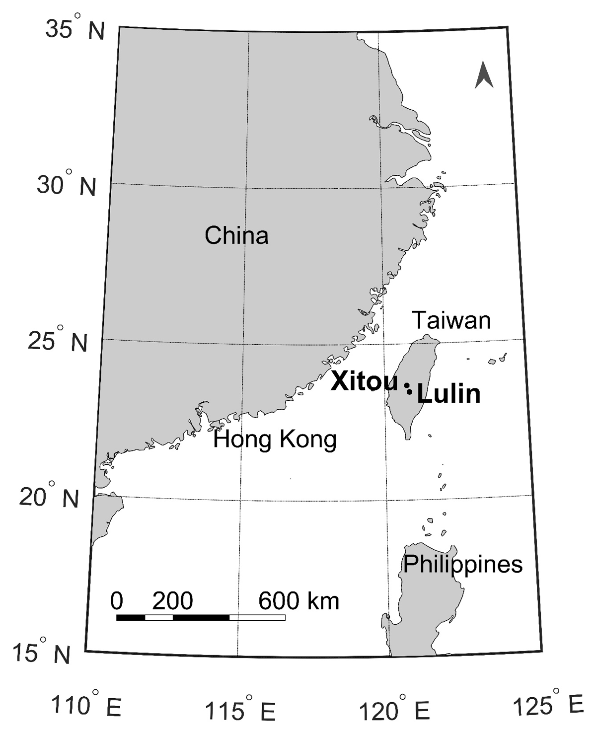
Figure 1
Map of the two study sites Xitou and Lulin in central Taiwan.
Lulin
The high mountain-top site Lulin is frequently above the atmospheric boundary layer in the free troposphere. Nearby the study site (50 km radius), there are only small villages at much lower altitudes. The nearest big city is Taichung, around 90 km southwest. The mountain slopes near the study site are covered with rather undisturbed forest. The average air temperature at Lulin is 10 °C, with the lowest monthly means of 5 °C in January and the highest means of 14 °C in July. The annual precipitation is variable and exceeds 4000 mm (Sheu et al., 2010). The fog collector system was installed on top of the Lulin Atmospheric Background Station (LABS) building, 6 m above ground level. The fog collector was oriented into the main wind direction, i.e. southwest (Fritz et al., 2021), to ensure undisturbed airflow.
We sampled during two intensive operation periods (IOP) at Lulin. The first IOP was in the wet season from 16 August 2018 to 04 September 2018 (19 days). We took 622 fog water samples and analysed 181 of them in the lab for their inorganic ion concentrations. The second IOP at Lulin was in the dry season from 08 March 2020 to 18 March 2020 (10 days). We took 498 samples and analysed 184 of them in the lab. This IOP period was very short due to the upcoming corona pandemic and related travel restrictions, but much foggier than the first IOP.
Xitou
The Xitou site is located in mountainous terrain in a coniferous forest dominated by Cryptomeria japonica (Wang et al., 2011). The highly industrialized area of central Taiwan is located at a distance of only 15 km to the west (Liang et al., 2009). The nearby surroundings of the Xitou site are mainly dominated by day tourists of the nature park. Additionally, the region is used for intensive agriculture, which is associated with the application of fertilizer.
The climate conditions are subtropical. The annual air temperature is 16.6 °C, with the lowest monthly means of 12.0 °C in January and highest means of 20.8 °C in July. The annual precipitation is 2235 mm. The wet season lasts from May to September, while the drier season occurs from October to April. The topography at the Xitou tower is relatively flat with a 15° slope. The valley is oriented south (top) to north (bottom). Fog and wind direction have a daily pattern at Xitou. Typically, a valley wind from the north forms around midday and is associated with the formation of fog due to adiabatic cooling of the advected air masses (orographic fog) (Chen, 2021). After sunset, the wind direction changes to a mountain wind from the south (Simon et al., 2016; Maneke-Fiegenbaum et al., 2018). The fog collector was installed at the tower at 37 m above the ground and oriented into the main wind direction during fog, i.e., the north, to ensure undisturbed airflow.
At the Xitou site, we operated one IOP that lasted from 26 July 2019 to 20 August 2019 (25 days). We took 98 fog water samples, all of which were further analysed in the lab.
Fog collection
The instrumentation includes a present weather detector that controls an active fog collector, a sample volume gauge, a magnetic valve, and an auto sampler (see Figure 2). The present weather detector (model PWD11, Vaisala OY, Finland) measured the visibility. Whenever the visibility dropped below 1000 m on a 10 minute mean basis, the fog collector was activated and the fog sampler started to collect water. The collection unit of the fog sampler is of a modified Caltech design (Degefie et al., 2015). It is completely made of inert materials: The unit itself is made of polyether ether ketone (PEEK), and the collection strings are made of polytetrafluoroethylene, better known as Teflon (PTFE), which is used to prevent any metal or ion contamination from the construction materials. All tubes and other surfaces that come into contact with fog water are also made of Teflon. The water level in the volume gauge is detected with a photoelectric sensor: the light transmission in air and water is different and therefore indicates whenever the sampling volume of 10 ml is reached. A magnetic valve opens and the sample is released into a standard laboratory auto-sampler (Model PS62, MLE GmbH Dresden, Germany), which is equipped with up to 109 centrifuge tubes (each 15 ml, HDPE). The system is operated with an Arduino microcontroller.
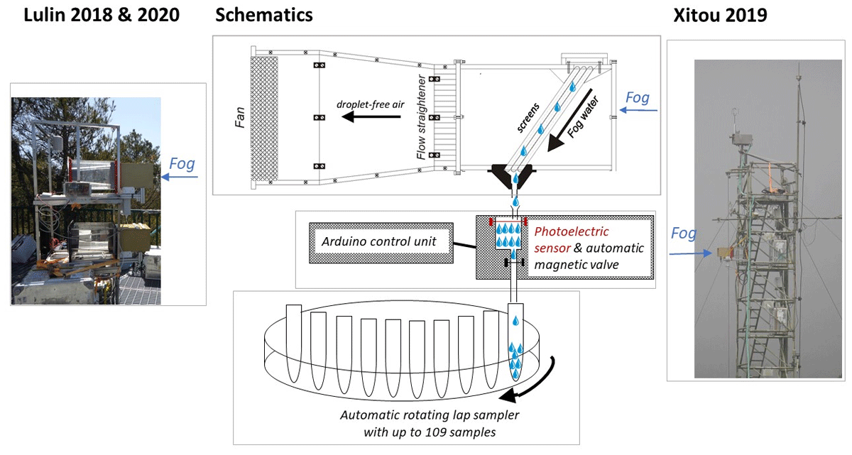
Figure 2
Photograph of the set-up at Lulin (left photograph), schematic sketch of the instrumentation (not to scale) and photograph of the setup at Xitou (right photograph: note the changed flow direction).
The setting is unique in that it is the first fog collection unit that collects subsequent samples based on a fixed volume of fog water. We decided on a volume of 10 ml per sample, as this volume was sufficient for analyses and allowed us to collect fog water on a rather short sampling period, sometimes less than 1 minute, depending on the liquid water content (LWC) of the fog. During the field campaigns, all samples were filtered as soon as possible after collection with a 0.2 µm pore size string Teflon filter. Electric conductivity and pH were measured in sample aliquots of 3 ml. This subsample volume was then thrown away and not used for further analysis. The other 7 ml were stored in a freezer (15 ml, HDPE) until further laboratory analysis with ion chromatography.
A strict cleaning routine was performed during the field campaigns. The fog collector, including the magnetic valve, all tubes and the auto-sampler, were cleaned with deionized water at least every other day and after each fog event. We expected that neighbouring samples would be more similar in conductivity and pH values than samples further away from each other, as shown by other studies (Simon et al., 2016; Nieberding et al., 2018). In addition, the compositions of neighbouring samples are likely to be more similar to each other than to those of other samples or to that of de-ionized water. Accepting the very low risk of cross-contamination or cross-dilution, a filter was used for several subsequent samples. The electrodes (conductivity and pH) were not cleaned between the samples but were fully drained. Following the reasoning described above, any cleaning with pure water could introduce a dilution effect, which we considered to be more serious than the risk of the carry-over effect. Therefore, we decided to clean the equipment between samples of different events, but not between samples of the same event.
The first sample normally has a longer sampling period than following samples, because all materials need to be wetted before the water drops down into the sampling bottles. Thus, the LWC is slightly underestimated in the first samples. Whenever a sample is taken, the amount of water leftover inside the collector and tubes is around 10%, which creates a carry-over effect between neighbouring samples. Note that the carry-over effect should not reach farther than one subsequent sample. After termination of a fog event, all laboratory material was cleaned with deionized water, dried and put into storage.
We took blank samples of the deionized water for quality assessment and quality control (QA/QC). For laboratory blanks, deionized water was filtered with previously used filters and with new filters. Field blanks were taken after the fog collector was cleaned, blanks were collected by spraying deionized water into the fog collector and collecting it in the same way that real fog water samples were collected. All blanks showed low conductivity, and the pH values also showed no indication of contamination.
Chemical analysis
The ion chromatographic analysis was conducted at the Department of Atmospheric Science of the National Taiwan University after each of the three IOPs. The LWC was calculated for each sample with the fog water collection rate (FWCR, in unit mg min–1) divided by the product of fog collection efficiency (88%) and flow rate (17.23 m3 min–1) (Simon et al., 2016). The ion loads of ions i per volume of air (IL(i), in units μeq m–3) were calculated from the measured ion concentrations (IC(i)) in units μeq L–1) and LWC using:
where (i) represents the individual ion species and ρ is the density of water (1000 kg m–3).
Frequency analysis
A frequency analysis was applied to the meteorological data in order to quantify the spectral ranges of the predominant turbulent motion. A Fourier-transform decomposed the time series into a large number of sine and cosine functions. The frequencies and amplitudes of these functions describe the recurring changes of the meteorological parameters with time. This yields a frequency domain of meteorological parameter changes under study and determines the time domain within which the spectral density of turbulent motion was highest. In micrometeorological applications, this approach is used – among others – for data quality assurance (Burba, 2013). Here, we will compare the most relevant frequency domain with the time resolution of fogwater sampling. In order to capture the full spectrum of changes of LWC and ion concentrations, the sample collection should be made at least on the same frequency as the frequency of highest spectral density of turbulent motion.
Backward trajectories
We calculated air mass trajectories with archive meteorological data in order to develop an understanding about the origin of the air masses and the possible sources of pollutants. Backward trajectories (48 hours) were calculated with the Hybrid Single-Particle Lagrangian Integrated Trajectory model (Draxler and Hess, 1998; Stein et al., 2015; Rolph, Stein and Stunder, 2017) provided by the Air Resources Laboratory of the National Oceanic and Atmospheric Administration (NOOA) at https://www.ready.noaa.gov/HYSPLIT_traj.php. We used the Global Data Assimilation System (GDAS) with a 0.5 degree resolution for Lulin 2018 experiment. For the Xitou 2019 and Lulin 2020 experiments, we used the Global Forecast System (GFS) with a resolution of 0.25 degrees. This improved resolution was not available for the Lulin experiment in 2018.
Results and Discussion
First, we provide a general overview of our IOPs and the new instrumentation, then we show results of four selected fog events in detail. Moreover, we compare these results to those obtained with the traditional, fixed-schedule sampling method. Finally, we discuss the origins of the foggy air masses.
Fog frequency and sampling period
An overview of all IOPs is given in Table 1. During the summer campaigns (Lulin 2018 and Xitou 2019) we had large data losses due to heavy rain that caused power outages and precautionary shutdowns. We presume that the losses of fog-related data are minor. The fog frequency was, in general, somewhat higher at Lulin than at Xitou. The percentage of fog days (minimum 1 hour of fog per day) was 80% – 90% at Lulin and 70% at Xitou, which is within the range of earlier studies at the same sites (Simon et al., 2016; Breuer et al., 2021). The main technical goal of all three IOPs was to collect as many back-to-back samples as possible within single fog events. Therefore, we aimed for long events with a minimum of 8 subsequent samples (Table 1). These events lasted between 1.5 and 13 hours (median 4 hours).
Table 1
Overview of the tree IOPs with statistical information of the fog water samples. Long events include a minimum of 8 subsequent samples. Lab samples are those selected for ion analysis in the laboratory.
| LOCATION | MEASURING PERIOD | DATA LOSSES | FOG FREQUENCY | NUMBER OF SAMPLES | NUMBER OF LAB SAMPLES | LONG EVENTS |
|---|---|---|---|---|---|---|
| Lulin | 16.08.2018 to 04.09.2018 (19 days) | 37% | 38% | 622 | 181 samples from 3 events | 12 |
| Xitou | 26.07.2019 to 20.08.2019 (25 days). | 27% | 11% | 98 | 98 samples from 7 events | 6 |
| Lulin | 08.03.2020 to 18.03.2020 (10 days) | <1% | 39% | 498 | 184 samples from 4 events | 6 |
During the 24 long events (Table 1), we sampled 837 samples at a median collection period of 3 minutes, 45 seconds (Figure 3). Compared to other studies (Simon et al., 2016; Nieberding et al., 2018), this is an order of magnitude shorter sampling period than previously achieved sampling frequencies. Overall, 90% of the samples were collected in under 12 minutes, which is less than half of the collection period than that achieved with the traditional sampling routine.
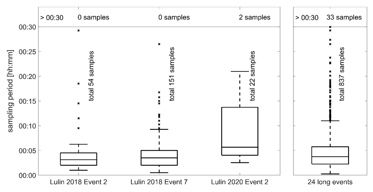
Figure 3
Boxplots of sampling periods of three longer events later discussed in detail, and of all samples of the 24 long events.
Different event types
We describe four different events of our IOPs that represent four different meteorological conditions.
Advective fog event during the wet season
The wet season at Mount Lulin is dominated by frequent rain and fog, sometimes in combination with each other. Consequently, the atmosphere was rather clean and the electric conductivity of fog samples (median 18.5 µS cm–1) was low compared to that of earlier studies at the same study site (median 103 µS cm–1, Simon et al., 2016). Nevertheless, the first event started at a relatively high conductivity of 99.5 µS cm–1 and a low pH of 3.85 at 01:00 LT. Dense fog formed and the visibility remained low for the next two hours (Figure 4a). As early as during the first hour of the event, the conductivity decreased and the pH increased (Figure 4b). For the next hour (02:00 LT to 03:00 LT), there was little change in conductivity, and the pH remained relatively constant at about 4.5. The LWC increased and decreased later, with a well-pronounced peak just after 02:00 LT (local time, which is UTC + 8 hours) (Figure 4c). The concentrations of inorganic ions dropped synchronously with the conductivity (Figure 4b & 4c) and also increased towards the end of the event. The chemical composition was clearly dominated by H+ (about 25%), NH4+ (about 15%), SO42– (about 25%) and NO3– (about 10%), which account for around 75% of the total ion concentration during the whole event. Former studies at the study site indicated that these four ions make up more than 85% of the total ion composition (Simon et al., 2016).
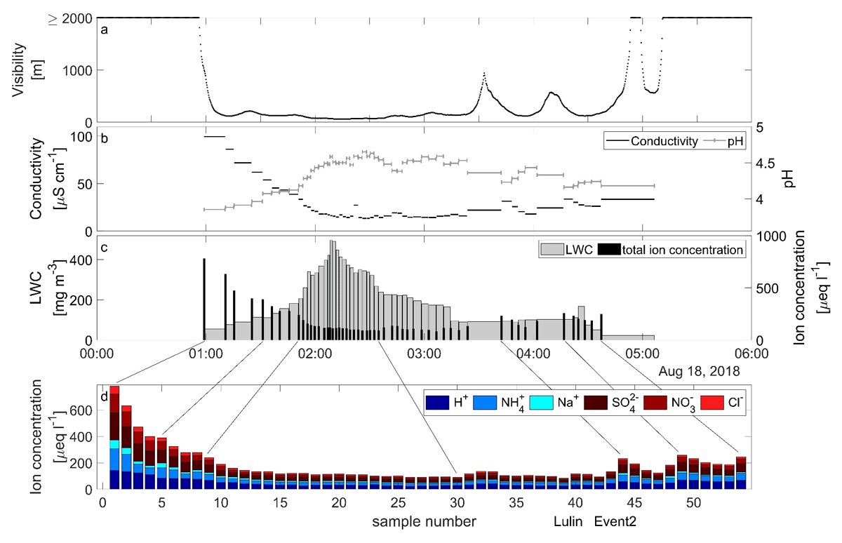
Figure 4
Time series of the fog event on the 18th of August 2018 at Lulin, showing (a) the visibility, (b) the conductivity and pH, (c) the LWC, and (d) ion concentrations.
The median sampling period for this event was 3 minutes and 8 seconds; the shortest sampling period was only 1 minute (Figure 3). According to spectral analysis (Fourier transform), the highest turbulence intensity was associated with eddies lasting between 5 seconds and 2 minutes. Therefore, our sampling method was not quite able to fully capture the turbulent changes. Related to the wind speed (median 1.45 m s–1), a sample within the median sample period could cover a cloud cross section of 270 m, the shortest sampling period showed a spatial resolution of around 90 m.
During this specific fog event, we presumably observed the passage of an advected cloud. At the edges of the cloud, which correspond to the beginning and the termination of the fog event at the fixed sampling site, we observed low LWC and thus higher concentrations of ions, high conductivity and low pH. During the centre of the event, which corresponds to the centre of the moving cloud, the foggy air mass was rather homogenous. The phase-out period of the event was less pronounced than the initial phase, which showed rapid changes of all measured chemical parameters.
Advective fog during the dry season
An advective fog during the dry season, showed quite different dynamics. Although it occurred during the dry season, it started with heavy rain and low visibility (Figure 5a). We had refrained from sampling fog during rain, because during such conditions rain enters the fog collector, hindering a clear discrimination between rain and fog droplets. Therefore, the fog sampling started in the middle of a cloud. At the sampling site, the cloudy (foggy) conditions lasted another 6 hours after termination of the rain. The conductivity was rather low in the beginning of the sampling period, well below 100 µS cm–1 (Figure 5b). A large portion of the aerosol particles carrying the inorganic ions had been washed out by the rain before the onset of the sampling, so only a low level of air pollution remained. The conductivity increased during the event, and later on the fog was less homogeneous (Figure 5a), and the conductivity was more variable during this period (15:00 LT to 18:00 LT). However, the pH was lower (below 4 throughout) than in the event described above and it decreased during the event (Figure 5b). The total ion concentration followed the shape of the conductivity curve (Figure 5c). The dominating ions again were H+ (about 20%), NH4+ (about 30%), SO42– (about 20%) and NO3– (about 15%), summing up to about 85% of the total ion equivalent concentration, which matches well the results of former studies during the dry season (Simon et al., 2016). The LWC was above 200 mg m–3 in the beginning and decreased more or less continuously with time down to around 15 mg m–3. The turbulent energy for this event peaked at somewhat longer timescales (10 seconds to 5 minutes). The median sampling period was 5 minutes and 38 seconds (Figure 3), and the shortest sampling period was taken in 2 minutes and 32 seconds. As such, this median sampling period was again close to catching the turbulent changes. The wind speed during this event was quite high, with a median of 4.36 m s–1, so that the median sampling period corresponded to a cross section of about 1.5 km within the cloud (around 600 m for the shortest sampling period). Accordingly, these samples still cover a wide range of changing meteorological conditions. We assume that we probed an advective cloud in this case, with edge effects evident at the end of the fog event.
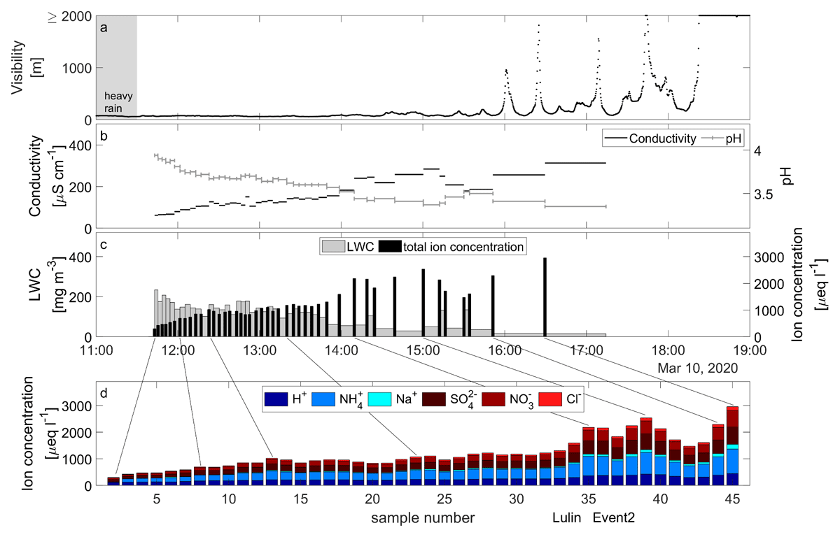
Figure 5
Time series of the fog event on the 2nd of March 2020 at Lulin showing (a) the visibility, (b) the conductivity and pH, (c) the LWC, and (d) ion concentrations.
Long event during wet season
The third event of this study site represents a very long fog event during the wet season. Heavy rain occurred before the event, then very dense fog with a visibility below 200 m was measured for around 8 hours onwards, followed by intermittent fog for around 4 hours (Figure 6a). A total of 151 samples were taken during this event. The conductivity (Figure 6b) was very low throughout the event (<25 µS cm–1); slightly higher conductivity only occurred in the middle of the dense fog (13:00 LT to 16:00 LT, >15 µS cm–1), and from 17:00 LT on it was very low (<10 µS cm–1). The pH was more variable through the event (Figure 6b). The first sample was rather high with a pH of 5.29, whereas the next sample (pH 4.56) and the following one were more acidic. One higher pH value (5.1) was measured around 12:20 LT. All other samples until 18:00 LT were below 5. Later on, the pH increased and fluctuated between pH 5.0 and 5.5, except for three samples that jumped up by at least 0.45 units compared to the neighbouring samples (19:40 LT, 19:46 LT and 22:40 LT). Compared with former studies during the same season at the site (Simon et al., 2016), in our samples the pH was high and the conductivity very low. The LWC (Figure 6c) can be categorized into three stages: 12:00 LT to 17:45 LT (median LWC 147 mg m–3), 17:45 LT to 19:53 LT (median LWC 357 mg m–3), and 19:53 LT to 23:11 LT (median LWC 83 mg m–3).
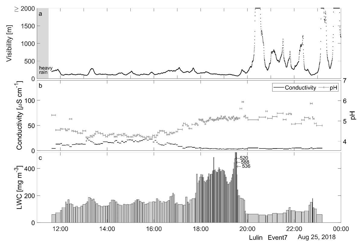
Figure 6
Time series of the fog event on the 25th of August 2018 at Lulin showing (a) the visibility, (b) the conductivity and pH, and (c) the LWC.
The turbulent energy peak during this event was similar to that of the last event (10 seconds to 5 minutes). The median sampling period was around 3 minutes and 30 seconds, with the shortest sampling period being 30 seconds. Along with the median wind speed (0.78 m s–1), the air mass moved about 160 m during the median sampling period, 23 m for the shortest sampling period. Our sampling routine was, thus, within the same temporal domain as the turbulent advective processes of the fog. Note that this event also represents orographic fog. The sampling started in the middle of the foggy (cloudy) air mass with very low visibility. Around 20:00 LT, the fog was less homogeneous, and towards the end of the fog event, the edge effects became evident. The ion composition was not measured for this event, as the number of samples would have exceeded the laboratory capacity.
Shorter event during wet season
The shortest event discussed in this paper occurred at the study site Xitou during the wet season. It lasted only 1.5 hours but still included 22 samples. In the upper panel of Figure 7, the data of the automatic sampling routine is shown (Figure 7a & 7b). During this event we had some data storage issues, so, the visibility data is not shown here. This location, at a lower elevation than the Lulin site, is more affected by regional air pollution (Liang et al., 2009; Simon et al., 2016). Therefore, the conductivity and ion concentrations were higher compared with the other events. The conductivity started at 649 µS cm–1 during the onset of fog and decreased afterwards (Figure 7a). After the 10th sample (69 minutes), the conductivity slightly increased. The pH was relatively high (4.89) and even increased during the event up to pH 6.21. The ion concentrations followed the shape of the conductivity curve (Figure 7b). The chemical composition was somewhat different compared with that of the other study site: Here H+ only played a minor role. The dominating ions were NH4+ (about 45%), SO42– (about 20%) and NO3– (about 20%), summarizing to 85% contribution to the total ion composition. In former studies, H+ ions also had a less dominant effect on the total ion composition for this study site (Simon et al., 2016), yet our values are really low. The turbulent energy peak during this event was in the same range as the other events (between 5 seconds and 5 minutes). The median sampling period for this event was around 4 minutes; thus, this resolution only covers a small portion of the turbulence elements. The median wind speed during this event was around 0.6 m s–1, such that the air mass moved 150 m during the time a sample was taken. This sampling period was not short enough to show all changes of meteorological processes. Other studies estimated that the droplet growth time was around 23 seconds (from diameter 0.25 µm to 17.33 µm) for the study site (Baumberger et al., 2021); therefore, the sampling period was rather long compared to the timing of other relevant processes.
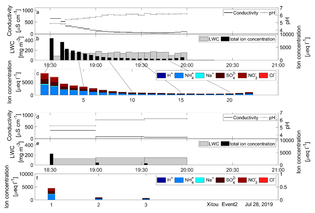
Figure 7
Time series of the fog event on the 28th of July 2019 at Xitou, showing the original samples in the upper panels for (a) conductivity and pH, (b) the LWC and total ion concentration, and (c) the ion concentrations. Averaged samples to approximate a traditional sampling procedure are shown in the lower panels for (d) conductivity and pH and (e) the LWC and total ion concentration, and (f) the ion concentrations.
Comparison of short sampling period and traditional sampling routines
So far, we have shown that the chemical composition of fog water changes quickly during various fog events, and we were able to determine this by using our newly developed sampling routine, which takes a sample whenever 10 ml of fog water has been collected. We observed rapid changes, especially during the very early and the very late stages of fog events. In this section, we show the difference between the traditional sampling procedure and the new routine.
The traditional sampling procedure is based on fixed time intervals: At the fixed time intervals (typically 30 min), an operator manually checks, whether the required water volume (typically 30 ml, due to historical laboratory capacities) is reached. When the required sampling volume is reached, the sampling bottle is changed; otherwise, the sampling continues for another 30 minutes (Sträter, Westbeld and Klemm, 2010; Degefie et al., 2015; Simon et al., 2016; Nieberding et al., 2018). For the comparison presented here, we merged our short sampling period to simulate a traditional sampling schedule with 30 minute intervals. We computed volume weighted averages of the ion concentrations of samples within 30-min sampling intervals. The respective pH’s were calculated from a volume weighted means of the H+ concentrations. This routine was applied for the event on 28 July 2019 at Xitou.
The upper panels of the Figure 7 was described before: It shows the data of the new automatic sampling routine (Figure 7a & 7b), while the (computationally averaged) results of the traditional sampling procedure are displayed in the lower panels (Figure 7c & 7d). For this analysis, the volume-weighted average concentrations were calculated while the pH was calculated from a volume-weighted mean of the H+ concentration. The original 22 samples were averaged into only 3 samples (Figure 7c and 7d).
We still see the decrease of the conductivity with time and an increase of the pH (Figure 7c), but the steepness of both the decrease of the conductivity and the increase of the pH are lost. When viewed using the traditional sampling routine, the increase of the conductivity towards the end of the event (Figure 7a) is no longer apparent (Figure 7d). Further, the LWC seems homogeneous during the fog event (Figure 7d), and the decrease of the LWC towards the end of the event, which is shown in the original samples (upper panels), is no longer visible either. Also, the ion concentrations are flattened to a more homogenous level, in which only the first averaged sample is somewhat higher than the subsequent ones (Figure 7d).
To summarise, the traditional sampling procedure shows less variability, fewer changes and fewer peaks, in which all parameters became flatted and more homogenous and information was lost. The new sampling method shows more rapid changes, and the temporal resolution is sufficient to capture many of the quick changes that accompany meteorological conditions.
Trajectories and sources
The chemical composition of fog water is related to the origins of air masses and pollutants along their trajectories. Therefore, backward trajectories were calculated for all presented events (Figure 8). The trajectories for all samples of the event 2 of Lulin during the wet season 2018 (Figure 8a), are similar to each other, and the transport distance was around 1000 km within the preceding 48 hours (around 5 m s–1). The air masses only moved above the ocean, which led to considerable concentrations of Na+ and Cl– (Figure 4). For the following event of Lulin 2018 (Event 7, Figure 8b), the air movement was much slower (400 km in 48 hours, about 2.3 m s–1). This event was also dominated by sea salt (Figure 6). The event of Xitou 2019 (Figure 8c) shows trajectories arriving from an eastern direction. The air masses moved first above the ocean and afterwards above Taitung city (south east of Taiwan) and took up air pollutants, which led to higher ion concentrations and conductivity than at the other events (Figure 7). The air masses passed over the high mountains located east of Xitou: They underwent adiabatic lifting, and it is likely that some components had been washed out by rain before the air masses arrived at Xitou. The travel distance over the previous 48 hours was similar to that of the event presented before (around 400 km, about 2.3 m s–1). The last presented event of Lulin 2020 was the only event affected by air masses moving above mainland China, Taipei and the industrialized western lowlands of Taiwan (Figure 8d). The conductivity (Figure 5b) was much higher than during the other events at the same study site. The samples also might have been affected by seasonal biomass burning (Lin et al., 2014).
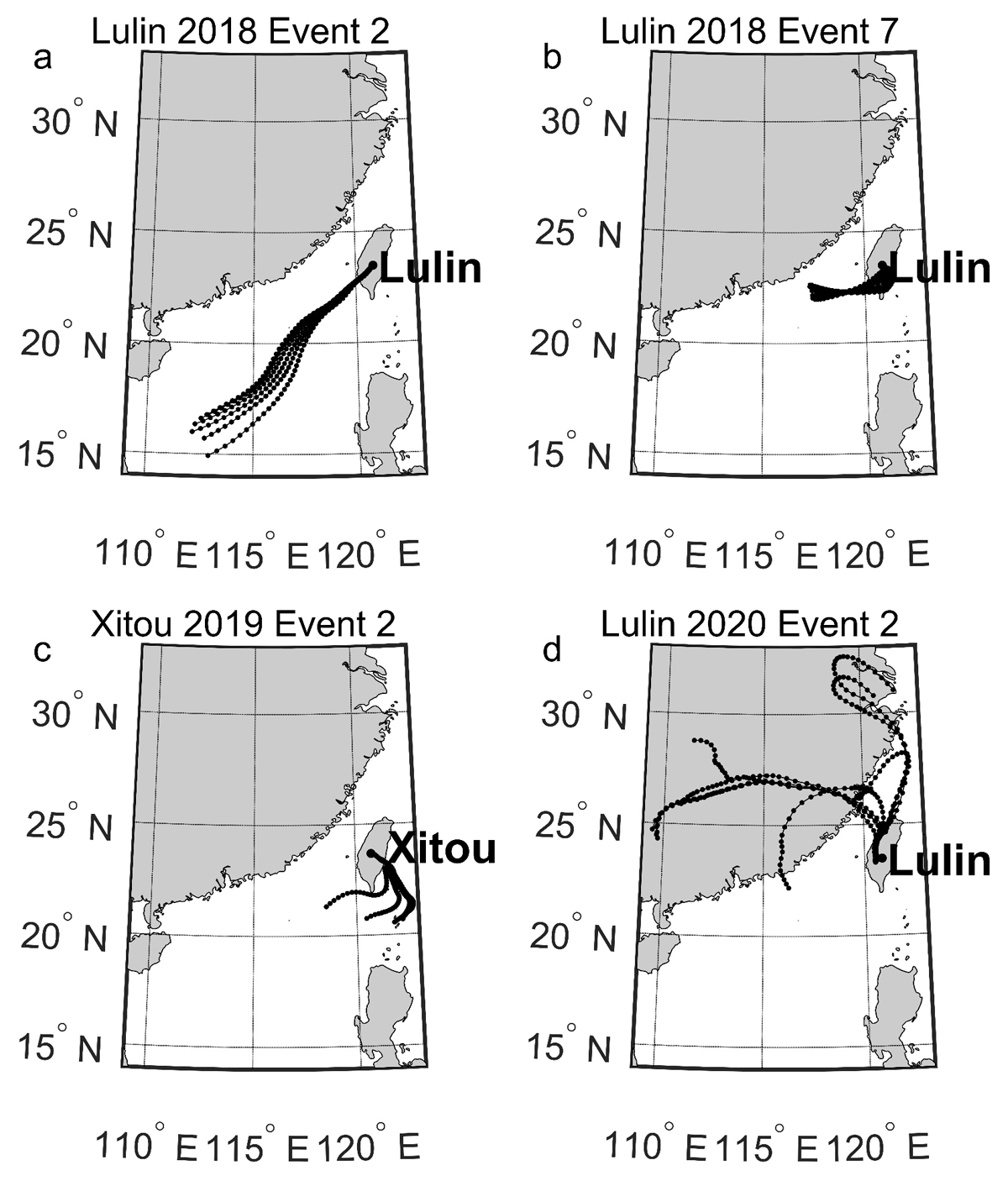
Figure 8
Backward trajectories of the last 48 hours before arrival at the study sites for the full time of the fog events at (a) Lulin, 18th of August 2018, Lulin, (b) 25th of August 2018, (c) Xitou, 28th of July 2019 and (d) Lulin, 2nd of March 2020.
Conclusion
The study took place at two mountain study sites in Taiwan, Lulin and Xitou, and used a new volume-based method for fog water sampling. The fog collector (modified Caltech design) was combined with a volume gauge, an automatic magnetic valve and an auto-sampler, taking samples whenever a volume of 10 ml of fog water was reached. Rapid changes of pH, conductivity and chemical composition could be shown during several events. With this new technical system, the median sampling period was only 3 minutes, 45 seconds. Changes of LWC and ion concentrations occur because of advective air masses with changing physical and chemical conditions. The samples at Lulin were mainly affected by long-distance transport, whereas the samples at Xitou were more affected by regional air pollution. When only a 30-minute sampling resolution to collect fog samples is possible, the observed changes in pH, conductivity and chemical composition are blurred or lost. Notably, the intra-event variability of pH, conductivity and chemical composition was larger than the inter-event variability.
To summarise, being able to achieve fog samples with a better time resolution is useful for showing the variability in the physical and chemical conditions within fog events. The highest variability in these conditions typically occurred during fog formation and fog dissolution phases, while the centre of the cloud (fog event) was rather homogeneous. In any case, the higher sampling frequency allowed for more detailed results.
Overall, according to the spectral analysis, our setup was not quite fast enough to cover most temporal regimes relevant for the dynamic processes in fog. In some cases (events 2 and 3, Figures 5 and 6) our sampling method mostly captured the variability of the physical and chemical conditions during fog rather well, while in other fog events our temporal sampling resolution was – relatively speaking – quite low.
Another issue is the relatively low sampling volume of 10 ml per sample in comparison to the leftover volume of fog water within the tubes and the collection system. This leads to a carry-over effect on the order of about 10% of the sample volume. We recommend that further instrument development should focus on minimising of these leftover volumes within the sampler while reducing the volume needed for laboratory analyses.
Further automation of on-site analyses (filtering, pH and electric conductivity) as well as the introduction of on-site ion chromatography would involve a rather complex extension of the experimental setup but would be accompanied by a significant reduction of the operator’s workload. The collection unit on the basis of the active string collector proved useful for the purpose our study. Last not least, the setup should be employed in radiation fog studies to develop further insight into the chemical dynamics of these systems.
Acknowledgements
We thank numerous students as well as staff members of Lulin and Xitou for their active support. We further thank C. Brennecka for language editing of the manuscript. The authors gratefully acknowledge the NOAA Air Resources Laboratory (ARL) for the provision of the HYSPLIT transport and dispersion model and READY website (https://www.ready.noaa.gov) used in this publication.
Funding Information
This work was supported by the German Federal Ministry of Education and Research under Grant DAAD [PPP 57447533] and Ministry of Science and Technology MOST (ROC) under Grant [108-2911-I-002-512].
Competing Interests
The authors have no competing interests to declare.
Author contributions
B. B.: Methodology, Software, Validation, Formal analysis, Investigation, Data curation, Writing-original draft, Visualization, N.-H. L.: Investigation, Resources, Funding acquisition, W. T.: Investigation, Resources, Funding acquisition, Y.-J. L.: Investigation, Resources, Funding acquisition, O. K.: Conceptualization, Methodology, Resources, Writing- review & editing, Supervision, Project administration, Funding acquisition.