
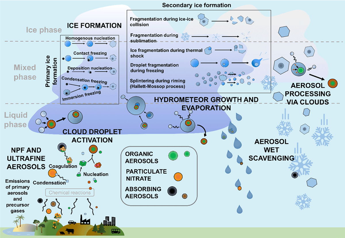
Figure 1
Visualisation of the aerosol and cloud processes targeted within FORCeS, including organic aerosol, particulate nitrate, absorbing aerosols, ultrafine aerosols and new particle formation (NPF), as well as cloud droplet activation, hydrometeor growth and evaporation, ice formation and aerosol processing and scavenging by clouds.
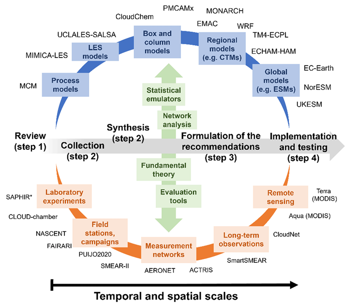
Figure 2
Schematic illustrating the overall approach, methodology and data within the FORCeS project. The timeline of the project is illustrated with grey arrows and steps from 1 to 4. The work within FORCeS has covered different temporal and spatial scales by utilising both models (shown in blue at the top) and observations (shown in orange at the bottom). Observations and models were intertwined with various analysis tools illustrated in the middle with green.
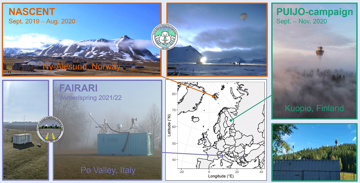
Figure 3
Overview of the in-situ measurement campaigns conducted within FORCeS: NASCENT in Ny-Ålesund, Norway, FAIRARI in Po Valley, Italy and PUIJO-campaign in Kuopio, Finland.
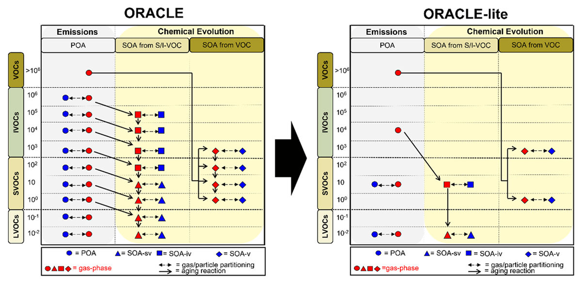
Figure 4
Schematic illustrating the difference between the full ORACLE (Tsimpidi et al., 2014, 2017) and ORACLE-Lite (Tsimpidi et al., 2025). Reproduced and modified under the Creative Commons 4.0 (CC 4.0) license.
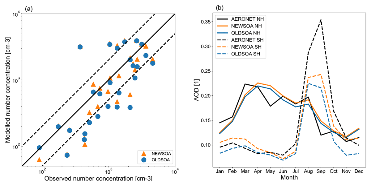
Figure 5
Evaluation of the performance between model simulations and observations presented in Bergman et al. (2022). Scatter plot in (a) shows the annual mean number concentrations at the stations (Table S3 in Bergman et al., 2022) in the year 2010, orange triangles indicate simulations with NEWSOA (online approach with lumped SVOCs and ELVOCs) and blue dots represent OLDSOA (offline calculation of SOA production). The black solid line shows the 1:1 line, and the dashed lines indicate a deviation of a factor of 2. Panel (b) shows the seasonal cycle of the mean AOD across all AERONET stations for Northern Hemisphere (NH, solid lines), and Southern Hemisphere (SH, dashed lines). Black lines indicate the derived AERONET AOD and the orange and blue colours are the NEWSOA and OLDSOA simulations, respectively. Figure adopted and modified from Bergman et al. (2022) under the Creative Commons 4.0 (CC 4.0) license.
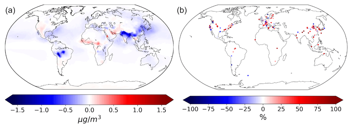
Figure 6
The change of the EMAC-simulated nitrate concentrations at surface after employing ISORROPIA-lite (vs. ISORROPIA II) is presented in (a), with blue colour indicating lower concentrations by ISORROPIA-lite. The coloured points in (b) show the deviations between EMAC results (with ISORROPIA-lite) and nitrate derived from observations with aerosol mass spectrometers around the world over the period 2000–2020.
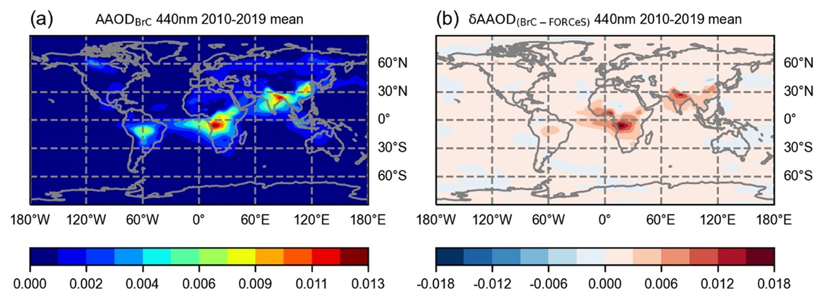
Figure 7
Absorption Aerosol Optical Depth (AAOD) for BrC at 440 nm is presented in (a). AAOD for BrC is calculated by the difference between two ten-year simulations, one accounting for BrC and the second one neglecting its absorption. In (b), the difference in AAOD at 440 nm between a simulation in which all OA is considered slightly absorbing (referred to as FORCeS) and a simulation where OA are only considered scattering and BrC only absorbing (referred to as BrC). Both subfigures display averages over ten-year periods (2010–2019).
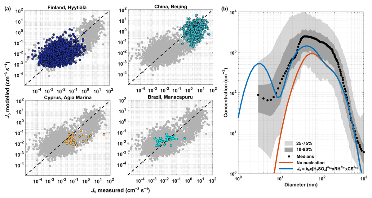
Figure 8
Preliminary J5 parametrisation testing results on several environment types involving boreal forests, giga-city, rural and rural/rain forest zone is shown in (a). Coloured points refer to the measurements at the specific sites and grey points show all measured data as presented in Li et al. (2025). The dashed lines are 1:1 line for the comparison between the measured and the modelled J5 values. In (b), TM5 simulation results for particle number concentration using Eq. (1) are shown as 2018 December medians (black dots and their shades) from pristine boreal forest, arctic remote boreal forest, urban, and rural regions as tests. “No nucleation” refers to no applied nucleation mechanism in TM5 simulation, and Eq. (1) showed promising prediction power, especially for particles at CCN size.
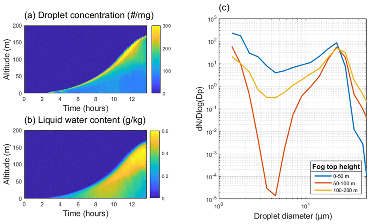
Figure 9
Example of the evolution of radiation fog. (a) droplet number concentration, (b) liquid water content, and (c) average fog droplet size distribution for the lowest 15 m during three different fog periods according to the fog top height. Simulations are conducted with UCLALES-SALSA (Sect. S3.1) in 2D setup employing the mean aerosol size distribution from the FAIRARI campaign (Sect. 2.2.3) and assuming constant aerosol hygroscopicity of 0.6. Vertical and horizontal resolution in the simulations were 1.5 m and 4 m. Atmospheric background sounding for initial conditions is typical for the nighttime radiation fogs observed in the area.
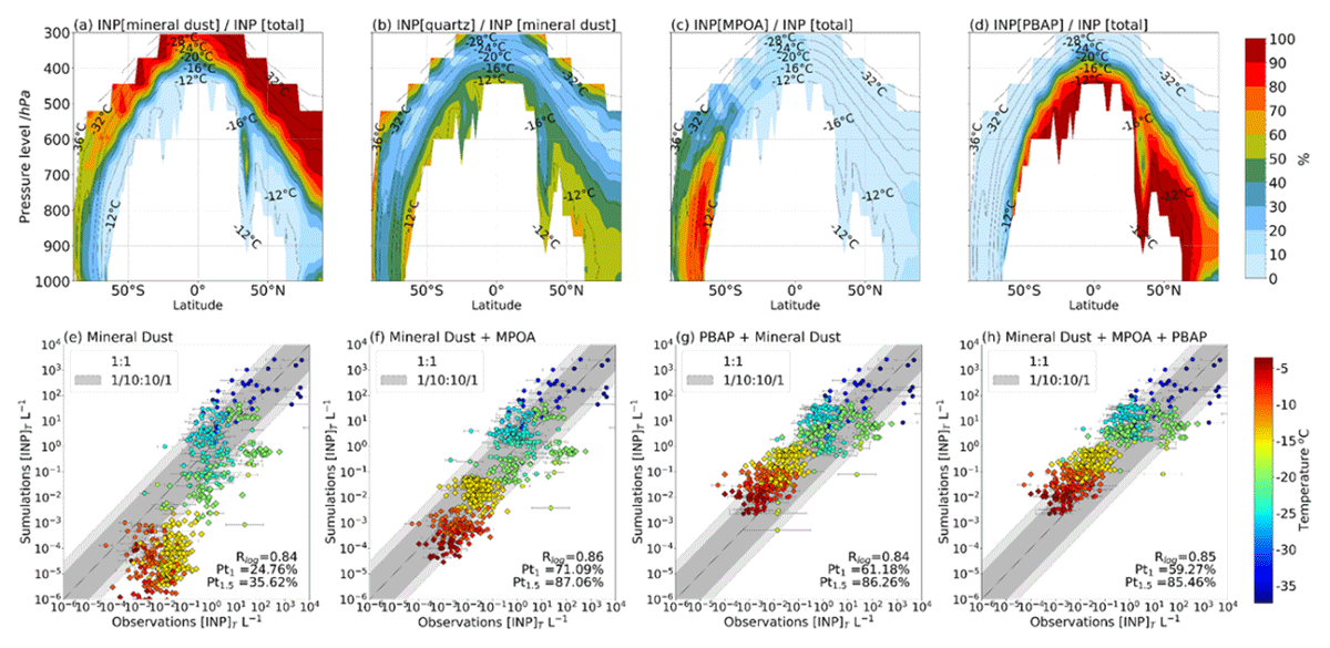
Figure 10
Top row: percentage contribution of each species to the total INP concentration (a–d), calculated using multi-year averaged zonal mean profiles of INP number concentration at modelled ambient temperatures. Panels show the contribution of: (a) quartz and feldspar, (b) the relative contribution of INP from quartz within the quartz and feldspar, (c) marine bioaerosols and (d) fungal spores and bacteria. The black contour dashed lines show the annual mean temperature of the model. Bottom row: Comparison of INP concentrations calculated at the temperature of the measurements against observations accounting for mineral dust (e), mineral dust and MPOA (f), mineral dust and PBAP (g) and all these combined (g). The dark grey dashed lines represent one order of magnitude difference between modelled and observed concentrations, and the light-grey dashed lines depict 1.5 orders of magnitude. The simulated values correspond to monthly mean concentrations, and the error bars correspond to the error of the observed monthly mean INP values. The colour bar shows the corresponding instrument temperature of the measurement in Celsius. Pt1 and Pt1.5 are the percentages of data points reproduced by the model within an order of magnitude and 1.5 orders of magnitude, respectively. Correlation coefficient is denoted with R, which is calculated with the logarithm of the values. Figure adapted from Chatziparaschos et al. (2025) under the Creative Commons 4.0 (CC 4.0) license.
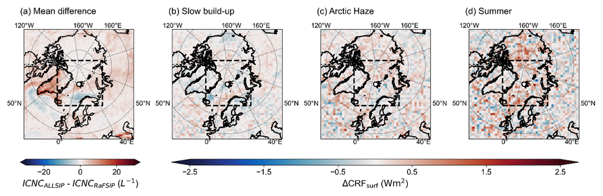
Figure 11
The first panel (a) shows the difference between mean ice crystal number concentrations predicted by the detailed microphysics simulation of WRF (ALLSIP) minus the simulation that ran with RaFSIPv2. The mean is derived from the entire year of simulations (September 2019–August 2020), focusing on the cases where: ICNC > 10–5 L–1 and temperature was between –25°C and 0°C (where ice multiplication was enabled in the WRF model). Panels (b) to (d) show the radiative biases in the predicted cloud radiative forcing at the surface calculated for the three periods: slow build-up (October–January), Arctic haze (February–May), and summer (June–September). Figure is adapted from Georgakaki and Nenes (2024) under the Creative Commons 4.0 (CC 4.0) license.
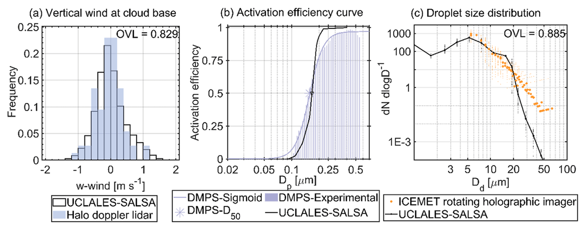
Figure 12
Modelled and observed cloud properties during the 5th hour of the cloud event of 24 September 2020 during the Puijo 2020 campaign. In (a), vertical wind at cloud base compared to Halo Doppler lidar observations is shown. Activation efficiency curve retrieved from Differential Mobility Particle Sizer observations with the twin-inlet system compared to modelled equivalent of total and interstitial aerosol particles is presented in (b). Droplet size distribution compared to observations with the ICEMET rotating holographic imaging system is shown in (c). Values of the overlapping index (OVL) have been added to indicate the degree of agreement between distributions. If two distributions are equivalent the OVL index tends to the unity.
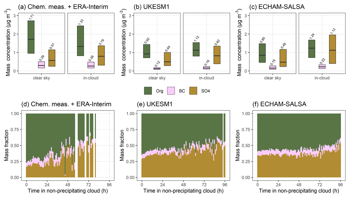
Figure 13
Top row: Median (black horizontal lines and numerical values) particle mass concentrations with 25th–75th percentiles (boxes) for OA (noted here, and in Isokääntä et al., 2022 as Org), eBC, and SO4 for the cold and polluted airmass sector at SMEAR II station, Hyytiälä, Finland. The experienced conditions by the air mass are denoted as clear sky and in-cloud (non-precipitating), and the data is temporally harmonised across observations and GCMs. Bottom row: The mass fractions of OA, SO4, and BC (derived from median concentrations at each 1-hour bin) for the more polluted air masses as a function of time spent in in non-precipitating cloud. Figure created from the data used in Isokääntä et al. (2022) and Talvinen et al. (2025).
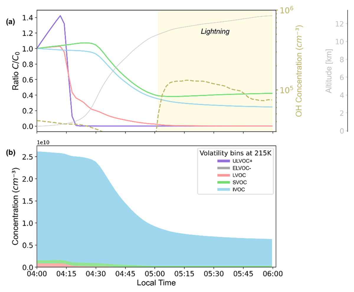
Figure 14
Transport of the isoprene gas-phase system during night-time convection over the Amazon. In (a) the fraction of the initial gas-phase concentration within volatility bins that survives night-time transport (chemistry and microphysics processes) is presented, and the altitude is shown with thin grey line and the OH concentration by the dashed olive yellow line. In (b) the contribution of different volatility bins to the total gas-phase concentration during transport is shown. Organic compounds are categorised according to their volatility with C* obtained for T = 215K: ULVOC+, extended ultra-low volatility organic compound, with the equilibrium saturation concentration C*(T) ≤ 3 × 10⁻⁷ μg m–3 (7 compounds) in purple; ELVOC-, reduced extremely low-volatility organic compound, with 3 × 10⁻⁷ < C*(T) ≤ 3 × 10⁻⁵ μg m–3 (1 compound = C4H5O3) in grey; LVOC, low-volatility organic compound, with 3 × 10⁻⁵ < C*(T) ≤ 0.3 μg m–3 (8 compounds) in red; SVOC, semi-volatile organic compound, with 0.3 < C*(T) ≤ 300 μg m–3 (1 compound = MVK/MACR = C4H6O) in green and the IVOC, intermediate volatile organic compound, with 300 < C* (T) ≤ 3 × 10⁶ μg m–3 (1 compound = Isoprene = C5H8) in blue.