
1 Introduction
FORCeS (Constrained aerosol forcing for improved climate projections, https://forces-project.eu/, last accessed: 3rd January 2025) was a 23-partner European project that aimed to better understand and reduce the uncertainty in anthropogenic aerosol radiative forcing. Anthropogenic aerosols exert a net cooling effect on climate through aerosol-radiation interactions (ARI, also referred to as the aerosol direct effect) and aerosol-cloud interactions (ACI, also referred to as the aerosol indirect effect) particularly by acting as cloud condensation nuclei (CCN) or ice nucleating particles (INPs) and influencing the properties of clouds. Increases in anthropogenic aerosols since pre-industrial times have led to a cooling effect, described by the effective radiative forcing (ERF), estimated to be between –1.7 and –0.4 W m–2 (when calculated as a difference between 1750 and 2019, Szopa et al., 2021). Natural aerosols have also changed since pre-industrial times, either affected by anthropogenic impacts (e.g. land use change), changes in climate, or a combination thereof. However, pre-industrial aerosol emissions remain uncertain (e.g. Carslaw et al., 2013; Mahowald et al., 2024). For instance, atmospheric dust loading has increased by approximately 55 ± 30% producing an ERF of –0.07 ± 0.18 W m–2 (Kok et al., 2023). Changes in aerosols have partly masked the warming effect of greenhouse gases (Bauer et al., 2022; Forster et al., 2021; Quaas et al., 2022; Salvi, Ceppi and Gregory, 2022; Szopa et al., 2021). Uncertainty in ERF also arises from the complexity of simulating the relevant atmospheric processes within Earth System Models (ESMs), especially related to ACI (e.g. Jia et al., 2021; Kahn et al., 2023; Regayre et al., 2018), hindering our understanding of past and future climate (Knutti, Rugenstein and Hegerl, 2017; Stevens et al., 2016). In ESMs, most of the aerosol processes need to be parametrised—due to the computational cost—rather than resolved by equations based on physical principles. This poses a central problem as nonlinear processes occurring at scales that are unresolvable by ESMs are represented by average quantities within the model grid-box. To improve estimates of aerosol ERF, improved and observationally constrained descriptions of the key processes involving aerosols and clouds are therefore required. These descriptions should naturally be as simple as possible in the context of the available computational resources. The aerosol and trace gas processes within the scope of FORCeS (Figure 1) include the descriptions of organic aerosols, particulate nitrate, absorbing aerosols (including dust, black carbon and brown carbon) and ultrafine aerosol microphysics. FORCeS also targeted key cloud microphysical processes such as cloud droplet activation, hydrometeor growth, and hydrometeor dynamics, ice nucleation and secondary ice formation, and aerosol processing and scavenging by clouds. The targeted processes were selected based on an expert assessment of scientific knowledge gaps and past systematic investigations of the expected sensitivity of the ESM predictions to these processes (Carslaw et al., 2013; Kulmala et al., 2011). The choice of processes was therefore based on a combination of different perspectives including: 1) past systematic assessments of model sensitivities (see e.g. Carslaw et al. (2013); 2) identifying areas with considerable accumulated process understanding that had not made its way to ESMs; 3) processes that were perceived potentially important but missing from current ESMs (and therefore part of the structural model errors and not included in sensitivity assessments conducted to date); 4) feasibility of making substantial progress during the four-year lifetime of the FORCeS project (see Sect. 2 and Figure 2 for more details on the process). The processes covered and model developments recommended within FORCeS therefore represent a mix where the relative weight of these different perspective varies – ranging from potentially incremental to certainly significant and from highly ambitious to certainly feasible. Below we provide some essential background information on these key processes and give a short overview on how they are typically described in ESMs.
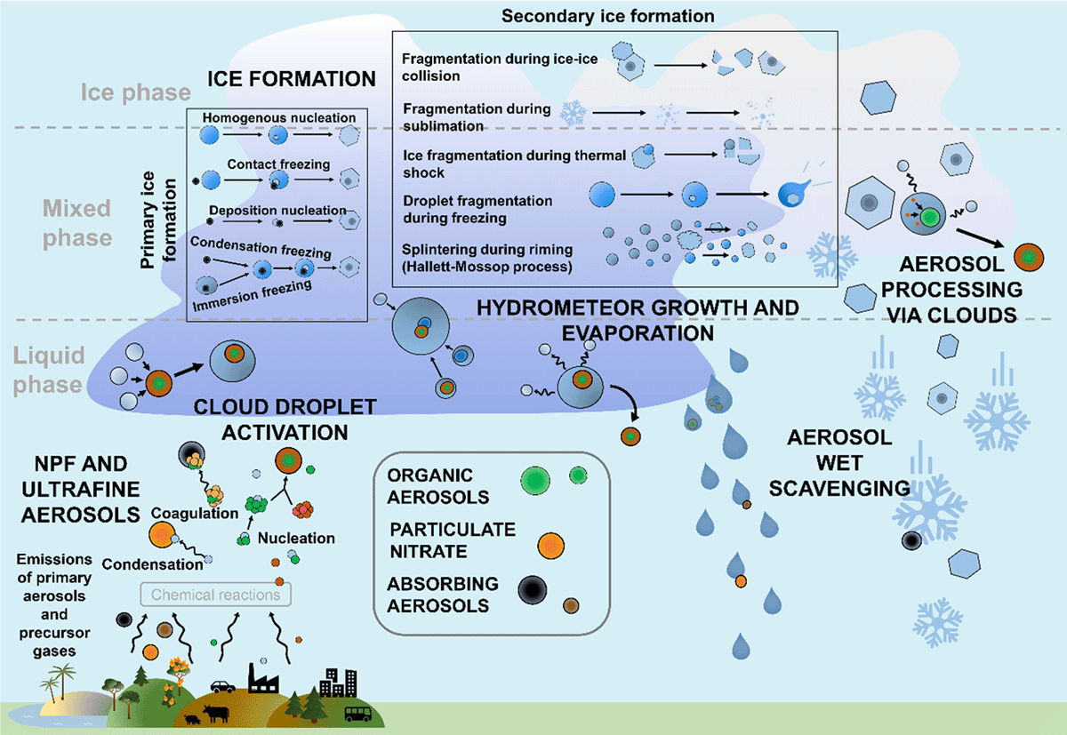
Figure 1
Visualisation of the aerosol and cloud processes targeted within FORCeS, including organic aerosol, particulate nitrate, absorbing aerosols, ultrafine aerosols and new particle formation (NPF), as well as cloud droplet activation, hydrometeor growth and evaporation, ice formation and aerosol processing and scavenging by clouds.
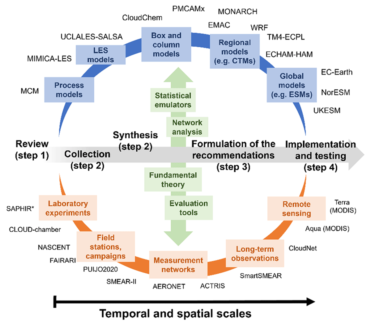
Figure 2
Schematic illustrating the overall approach, methodology and data within the FORCeS project. The timeline of the project is illustrated with grey arrows and steps from 1 to 4. The work within FORCeS has covered different temporal and spatial scales by utilising both models (shown in blue at the top) and observations (shown in orange at the bottom). Observations and models were intertwined with various analysis tools illustrated in the middle with green.
1.1 Organic aerosols
At least half of the sub-micrometre particle mass is comprised of organic compounds (17–92%, (Tsimpidi et al., 2025), which underlines the importance of accounting for organic aerosols (OA) in estimates of aerosol ERF (e.g. Shrivastava et al., 2017). However, despite the expansion in our understanding of OA processes during the last decade, models still struggle to reproduce the observed OA concentrations in certain areas (Ciarelli et al., 2016; Mao et al., 2018; Tsimpidi et al., 2016). First, uncertainties in emission inventories arise from the treatment of semivolatile (often called condensable) compounds at the emission source (Denier van der Gon et al., 2015; Simpson et al., 2020). Second, simulation of the production and evolution of atmospheric secondary organic aerosol (SOA) is challenging due to the complexity of the associated compounds, chemical reactions and microphysics (Shiraiwa et al., 2017). The descriptions of OA in ESMs can be improved through better accounting for e.g. the volatility distribution of the SOA species and their precursors. Furthermore, important feedbacks driven by climate impacts on the sources and sinks of OA are poorly constrained (Blichner et al., 2024; Tsigaridis et al., 2014; Yli-Juuti et al., 2021).
Organic aerosols have natural (e.g. biosphere, wildfires, sea spray) as well as anthropogenic (e.g. agriculture and various combustion processes) sources. A large fraction of the total atmospheric OA is secondary (Griffin et al., 1999; Kroll and Seinfeld, 2008), whose description requires knowledge about the emissions and concentrations of atmospheric volatile (VOCs) and intermediate volatility organic compounds (IVOCs), their oxidation within the atmosphere, and the volatility of the oxidation products – the latter determining the partitioning of various species between the gas- and condensed phases. Similarly, the primary organic aerosol (POA) components interact dynamically with the gas phase through condensation and evaporation upon transport and transformation in the atmosphere (Robinson et al., 2007). Consequently, the compounds contributing to atmospheric OA are often described using the volatility basis set (VBS) that approximates the complex mixture via surrogate species binned according to their effective saturation concentrations (Donahue et al., 2006, 2011).
Currently, the VBS framework is used to interpret laboratory experiments (Dada et al., 2023a; Stolzenburg et al., 2018; Tröstl et al., 2016) – for instance, to describe particle growth in field measurements (Mohr et al., 2019; Wang et al., 2024) – and it has been implemented in models with varying degrees of resolution (Farina et al., 2010; Irfan et al., 2024; Jiang et al., 2019; Liu et al., 2021; Tsimpidi et al., 2010, 2014). Within the atmosphere, OA components interact with each other, water (e.g. Carlton and Turpin, 2013; Fan et al., 2021; Voliotis et al., 2022) and other chemical species present in the particles (e.g. sulfates, nitrates, BC and crustal material (Li et al., 2021b; McFiggans et al., 2019; Zheng et al., 2020b). These interactions naturally add another dimension of complexity in understanding the evolution and impacts of OA.
The sources, properties and atmospheric evolution of the compounds present in atmospheric OA are important for the prediction of aerosol-cloud-climate interactions within ESMs (Kostenidou et al., 2018). Besides influencing the overall particulate matter (PM) loadings and the optical properties of the atmosphere (Zhu et al., 2023), the concentration and properties of OA components influence the aerosol number size distribution (He et al., 2021b; Zaveri et al., 2014) and hence the number of available CCN and INPs (Kuwata et al., 2013; Zheng et al., 2020a). Specifically, the representation of volatility is important for determining the ability of the organic species to contribute to new particle formation (NPF, see also Sect. 1.4) and nanoparticle growth (Riipinen et al., 2011, 2012; Stolzenburg et al., 2023). The aforementioned effects impact the quantification of the contribution of natural vs. anthropogenic aerosol influence on climate (e.g. Carslaw et al., 2013), including climate impacts of land-use change (e.g. Barati et al., 2023), or climate feedbacks involving forest-derived aerosols (e.g. Thornhill et al., 2021). Finally, the interactions of OA with atmospheric water are important for simulating the influence of aerosol perturbations on cloud microphysics and radiation directly, but also for the removal of OA from the atmosphere by wet scavenging (Hodzic et al., 2020; Holopainen et al., 2020).
The advances in our understanding of the processes related to OA during the last decades have not been fully exploited to advance the representation of the corresponding processes in ESMs. The simulation of SOA is challenging due to the multiple surrogate species that are required to represent the broad spectrum of chemical compounds relevant for OA (Curtius et al., 2024; Dada et al., 2023a; Ehn et al., 2014; He et al., 2021a; Pozzer et al., 2022; Shen et al., 2022, 2024; Wu et al., 2021). The ability of large-scale models and ESMs to reproduce the observed OA concentrations is highly variable (Kanakidou et al., 2005; Shrivastava et al., 2017; Sporre et al., 2020). In general, ESMs divide OA into primary and secondary, i.e. POA and SOA. However, the simulated sources, number of used surrogate compounds, chemical processing and assumed volatilitity distributions for the organic species vary widely among models. In some ESMs, SOA formation from anthropogenic sources is not explicitly represented; instead, the organic mass is emitted directly as primary particles, bypassing the intermediate oxidation and condensation processes. Also the treatment of the volatility of the OA components ranges from assuming entirely non-volatile and nonreactive OA to the description of OA with two volatility classes (e.g. Bergman et al., 2022). More advanced VBS representations with varying number of volatility bins are also available (Holopainen et al., 2022; Irfan et al., 2024) but rarely applied in fully coupled ESMs.
The global emissions of biogenic VOCs are usually described within ESMs using models that link land-use, terrestrial biota and environmental parameters. The Model of Emissions of Gases and Aerosols from Nature (MEGAN, Guenther et al., 2012) is an example of an emission model that is commonly used, and based on empirically driven emission factors for various land-use types. Another example is LPJ-GUESS which is a process-based dynamic vegetation and biogeochemistry model (Döscher et al., 2022 and references therein). VOC oxidation by OH and ozone is generally described by simplified chemical reaction schemes assuming, for example, constant SOA yields (Henze and Seinfeld, 2006; Hodzic et al., 2016; Tsigaridis et al., 2014). VOC oxidation by the nitrate radical is at present generally not accounted for in ESMs, with some exceptions, despite the potential large sensitivity of SOA formation from biomass burning emissions to this oxidation pathway (Kodros et al., 2020). Overall, ESMs still exhibit large uncertainty and systematic biases in terms of the coupling between temperature, VOC emissions, OA and cloud properties (Blichner et al., 2024). Furthermore, factors other than temperature such as CO2 concentration or stress due to drought or insect outbreaks, can also have a significant impact on VOC emissions (e.g. Faiola and Taipale, 2020; Holopainen et al., 2022; Holopainen and Gershenzon, 2010; Midzi et al., 2022), thus affecting the concentration of SOA and further aerosol radiative forcing (Bergström et al., 2014; Mentel et al., 2013). These, however, are rarely considered in the basic versions of ESMs.
1.2 Particulate nitrate
Inorganic ions such as sulfate (SO42-), ammonium (NH4+) and nitrate (NO3-) are major components of the atmospheric PM (Seinfeld and Pandis, 2016), and therefore have significant effects on ARI and ACI – not least due to their interactions with water (Burgos et al., 2020). Sulfate has received a lot of attention as probably the most important anthropogenic aerosol component during the industrial period (Ackerley et al., 2009; Nordling et al., 2021). The importance of understanding the sources, transport, atmospheric processing and effects of particulate nitrate has however become apparent in the recent years, given the decline in sulfate emissions and its links to land-use change and agricultural policies (Bauer et al., 2007; Xu and Penner, 2012). Ammonium nitrate is an important aerosol component in regions with intensive agriculture and traffic, such as China, western United States and western Europe (e.g. Highwood et al., 2012; Morgan et al., 2010) and its relevance is expected to increase in the future (Hoesly et al., 2018). Ammonium nitrate is also a key player in the atmospheric acid-base chemistry, which also has important implications for air quality and the deposition of nutrients (Baker et al., 2021; Kakavas and Pandis, 2021; Karydis et al., 2021; Nenes et al., 2021). Global ammonia emissions from agriculture are estimated to increase by 20–105% between 2000 and 2100 (van Vuuren et al., 2011). The conversion of gas-phase nitric acid to particle-phase nitrate is driven by ammonia, dust and salt minerals, influencing aerosol pH (Fenter et al., 1995; Karydis et al., 2016, 2021; Krueger et al., 2004; Milousis et al., 2024). Furthermore, the formation and properties of various organic nitrates have been the focus of research efforts in the past years (Bardakov et al., 2024; Graham et al., 2023).
Models still show significant spread in their estimates of nitrate levels. For example, the AeroCom phase III experiment (Bian et al., 2017) showed an average NO3– burden of 0.63 Tg among participating models, with an intermodal standard deviation of 0.56 Tg (nearly 90% of the mean), and extremes differing by a factor of 13. In an effort to balance precision and computational efficiency in the simulation of nitrate, a range of intermediate approaches have been proposed (Soussé Villa et al., 2025). One method involves simplifying the dynamic mass transfer equations to a first-order irreversible uptake process, which neglects the re-evaporation of absorbed species back into the gas phase (e.g. Fairlie et al., 2010).
Another approach is a hybrid strategy that applies thermodynamic equilibrium to fine (accumulation) modes or bins (Karydis et al., 2011), while using first order irreversible uptake (Hauglustaine, Balkanski and Schulz, 2014; Hodzic, Bessagnet and Vautard, 2006) or dynamic mass transfer (Capaldo, Pilinis and Pandis, 2000; Trump et al., 2015) for the coarse ones. A third option is to calculate equilibrium concentrations separately for fine and coarse particles, by first limiting the gas-phase material that can condense to each size bin or mode assuming diffusion limited condensation (Vignati et al., 2004) and then redistributing the mass between the gas and the aerosol phase, assuming instant thermodynamic equilibrium between the two phases (Karydis et al., 2016; Pringle et al., 2010). Although aerosol thermodynamic models are commonplace in regional chemical transport models, they are often absent in many ESMs, partly due to their computational cost. For example, versions of ECHAM (Roeckner et al., 2006; Tegen et al., 2019) do not simulate aerosol thermodynamics, and in NorESM1-M, using CAM4-Oslo, nitrate and its climate effects are not included (Kirkevåg et al., 2013). The CMIP6 (Coupled Model Intercomparison Project Phase 6, Eyring et al., 2016) version of EC-Earth3-AerChem (Sect. 2.1.1), on the other hand, employes the thermodynamic gas–particle partitioning model EQSAM (Metzger et al., 2002) to determine the partitioning of NH3/NH4+ and HNO3/NO3-, but applies this only for accumulation mode aerosols. ESMs typically assume a globally uniform dust composition, and organic nitrates are usually not explicitly simulated.
1.3 Absorbing aerosol: black carbon, mineral dust and brown carbon
The absorbing aerosol fraction comprises of black carbon (BC), dust aerosols and brown carbon (BrC) (Andreae and Gelencsér, 2006; Liu et al., 2015). A recent review estimated the fraction of absorbing aerosol optical depth to be 57%, 30% and 10% due to BC, dust and OA, respectively (Sand et al., 2021). Brown et al. (2021) showed that most climate models overestimate the absorption of radiation by aerosols from biomass burning. Recently, Zhong et al. (2023) also showed that climate model uncertainties in ERF can be reduced significantly by constraining biomass burning aerosols using observations and satellite data.
Eventually, the total absorption is derived from the sum of its components (see Figure 1 in Sand et al., 2021). The mixing state of aerosol also impacts the properties of absorbing aerosol (Kelesidis et al., 2022). An earlier study by Stier et al. (2007), however, found that the ESM absorbtion results are even more sensitive to the uncertainties in the imaginary index than to the mixing rules in their model setup. The absorption of mineral dust and carbonaceous aerosol is in general poorly characterised, which significantly contributes to uncertainty in the ARI (Bellouin et al., 2020; Bond et al., 2013; Kok et al., 2023; Regayre et al., 2023). Current ESMs treat BC and dust explicitly, but the absorbing fraction of OA is still unaccounted for, or represented with a simplistic approach as a very weakly absorbing aerosol (Hess, Koepke and Schult, 1998). The latter is therefore missing from the current IPCC estimates of radiative forcing. Better treatment of BrC could reduce the gap between results from ESMs and observations of aerosol absorption (Feng, Ramanathan and Kotamarthi, 2013; Jo et al., 2016).
Dust is emitted from the Earth’s surface through wind erosion processes. It consists of a mixture of minerals determined by the composition of the parent soil. These minerals have distinct physico-chemical properties (crystal structure, chemical composition), are often preferentially emitted in different aerosol sizes, and behave differently when exposed to radiation and clouds. For instance, iron oxides, hematite and goethite, dominate the absorption in the short wave (SW) range (e.g. Di Biagio et al., 2019; Engelbrecht et al., 2016; Moosmüller et al., 2012), while clays (e.g. kaolinite, illite, smectite) and coarse minerals, such as quartz or calcite, present the highest absorption features in the longwave (LW) range (Di Biagio et al., 2014, 2017). Dust is also estimated to be the most important INP in the global atmosphere, with K-feldspars and quartz likely being the most efficient sources of INPs relative to other minerals (Atkinson et al., 2013; Harrison et al., 2019; Zimmermann et al., 2008, see also Sect. 1.7) In addition, dust particles undergo chemical aging in the atmosphere, reacting with acids (such as sulfuric, nitric, or hydrochloric acid) or acquiring coatings of organic compounds (Goodman et al., 2001). The uptake rates of such compounds on dust are increased by the presence of calcite and other alkaline components (Kakavas and Pandis, 2021; Krueger et al., 2004). As a result of these coatings, dust absorption and hygroscopicity are modified (Milousis et al., 2025b; Usher et al., 2003).
Current ESMs typically assume that dust is a single species, neglecting the known regional variations in the mineralogical composition of its sources (Claquin et al., 1999; Green et al., 2023; Journet, Balkanski and Harrison, 2014). The explicit representation of certain key minerals in ESMs is more limited by our incomplete understanding of global soil composition and the associated size-resolved airborne mineralogy and optical properties than by computational constraints (Gonçalves Ageitos et al., 2023). In practice, this is translated into climate models specifying globally uniform imaginary parts of the dust refractive index, uptake rates and INP efficiencies. Furthermore, most ESMs underestimate the coarse and super-coarse dust fractions (Kok et al., 2021). Also, dust asphericity, which is neglected in most models, is estimated to enhance the dust mass extinction in the visible radiation by up to ~40% (Kok et al., 2017), which may be important for models to simultaneously match observations of optical depth and surface concentration (Kok et al., 2021). Currently, ESMs are often calibrated to achieve a global mean dust optical depth (DOD) of 0.03 ± 0.01 (Ridley et al., 2016). However, relying on this single constraint on the dust cycle leaves dust direct forcing efficiency underdetermined and thus makes room for a large range of plausible assumptions about mineral composition, size distribution, asphericity, and scattering among models. Consequently the CMIP6 ESMs diverged substantially in their dust direct forcing efficiency (Haugvaldstad et al., 2025). LW scattering of radiation by particles and molecules in the atmosphere is another effect that is typically neglected in models because absorption is the dominant process and including scattering would significantly increase computational costs. This omission leads to an underestimation of the LW radiative effects, particularly for coarse and super-coarse dust particles (Drugé et al., 2025; Kok et al., 2025). Finally, models are unable to simulate the increase in dust burden since the start of the industrial age as observed in dust sedimentary archives (Kok et al., 2023). The historical forcing by dust is therefore currently unaccounted for in estimates of ERF and climate sensitivity.
BrC has recently attracted enough attention to start being explicitly incorporated in global models (Zhang et al., 2020). To account for this additional aerosol absorption, most models simply include a small imaginary part to the refractive index of the organic aerosol (Tsigaridis and Kanakidou, 2018), implying that BrC is a constant fraction of OA worldwide. However, it is known that incomplete biomass burning and biofuel combustion, as well as secondary organic aerosol from the oxidation of aromatics, produce BrC with different proportions to organic aerosol (Basnet et al., 2024; Laskin, Laskin and Nizkorodov, 2015; Zhang et al., 2020). Furthermore, there are sources of OA that do not emit or produce measurable amounts of BrC. Variability in the absorption characteristics of BrC is attributed to emission sources and the molecular composition of BrC. Saleh (2020) categorised OA and the corresponding BrC based on their absorbing properties from very weakly (imaginary refractive index at 550 nm below 10–3) to strongly absorbing (imaginary refractive index above 0.1). Such large variability can be explained by the different fuels and combustion conditions resulting in BrC production. Navarro-Barboza et al. (2025) highlight the potential contribution of sources other than biomass burning or biofuel—including shipping and traffic emissions—to observed BrC absorption.
The atmospheric behaviour of BrC suggests the existence of two different primary BrC aerosol types, reactive and inert. Reactive BrC loses its absorbing properties by photobleaching (photolysis and reaction with OH) with an e-folding time of about 11 h during daytime (k = 3.4 × 10⁻⁵ s–1, Skyllakou et al., 2024; Wong et al., 2019). The inert type of BrC (estimated to be 6–10% of biomass-burning BrC, Forrister et al., 2015; Wong et al., 2019; Zhang et al., 2020) is removed from the atmosphere by deposition only. The presence of BrC also has implications on the photochemistry near the surface due to its nature to absorb at UV wavelengths (Mok et al., 2016). However, wildfire emissions may include “dark” BrC, which can also absorb in the visible light spectrum (Chakrabarty et al., 2023).
Most ESMs consider both internally and externally mixed aerosol, and typically apply the Maxwell-Garnett mixing rule for BC and dust present in mixtures (Sand et al., 2021). BC, released from various sources involving incomplete combustion (Rönkkö et al., 2023; Xu et al., 2021a), is currently considered in most ESMs and is estimated to exert a net warming impact on climate during the industrial period (e.g. Bond et al., 2013). Its total climate effect, however, is still uncertain due to uncertainties in the mixing state and cloud interactions of BC-containing particles. Current ESMs estimate the BC loadings within a order of magnitude (see e.g. Frey et al., 2021) but the agreement depends on the mass absorption coefficients (MACs) assumed when interpreting the data. For example, Sand et al. (2021) found large differences between the MAC values in ESMs, ranging from 3.1 to 17.7 m2 g–1 at 500 nm. Additional error sources are related to, for example, the coating and atmospheric ageing and scavenging of BC as well as the exact wavelength dependent function that describes the imaginary part of the refractive index or MAC.
1.4 Ultrafine aerosol and new particle formation
Atmospheric aerosol number concentrations are dominated by ultrafine (dp < 100 nm, Kwon, Ryu and Carlsten, 2020) particles (UFP). A large fraction of these particles are secondary, originating from NPF driven by atmospheric vapours (Kulmala, 2003; McMurry et al., 2000)—either in-situ in the atmosphere (e.g. Cai et al., 2024; Zhao et al., 2024) or upon emission from e.g. mobile sources (e.g. Kittelson et al., 2022). In NPF, vapour molecules collide and form small stable molecular clusters, which can then further grow by coagulation and condensation reaching sizes relevant (>20 nm and larger) for cloud formation (e.g. Dada et al., 2017, 2020; Kirkby et al., 2011, 2016, 2023; Kulmala et al., 2004, 2022; Lehtipalo et al., 2018; Wang et al., 2020; Williamson et al., 2019). Much progress has been made in recent decades to understand various processes and vapours leading to atmospheric NPF and their overall contribution to UFP and CCN numbers (e.g. Dada et al., 2023a; Dunne et al., 2016; Kirkby et al., 2023; Stolzenburg et al., 2023; Wang et al., 2023). NPF and the further condensation growth of the formed particles to sizes where they can contribute to ARI and ACI are complex processes that involve various atmospheric species such as sulfuric acid, ammonia, organics, iodic acid, etc.,—depending on location and atmospheric conditions (e.g. Baccarini et al., 2020; Kerminen et al., 2018; Zheng et al., 2020). Coagulation, which is strongly dependent on particle size and concentration, also plays a major role in modifying UFP concentrations, aerosol number size distributions and, hence, CCN levels.
Particle formation driven by sulfuric acid is probably the best documented NPF process, but it is well-known that various other species such as organic compounds, basic compounds such as ammonia and amines (Dada et al., 2023b; Yan et al., 2021), iodic acid (He et al., 2021a), nitric acid (Wang et al., 2020), water as well as atmospheric ions (Enghoff and Svensmark, 2008; Kirkby et al., 2011; Nieminen et al., 2011) can participate in NPF depending on the environment in question (e.g. Zhao et al., 2024). Long-term observations from the boreal forest in Hyytiälä show a decline in the NPF frequency and intensity over the past 25 years (Li et al., 2024c), potentially driven by the decrease in sulfuric acid following the decline of sulfur dioxide (SO2) from European sources. Meanwhile, less intense NPF events driven by highly oxidated organic molecules (HOM) from forest emissions have become more frequent (Kulmala et al., 2022). Also, laboratory studies such as the CLOUD experiment (see Kirkby et al., 2023 and Sect S4.1) and experiments in the SAPHIR chamber (Sect. S4.2) have investigated various systems relevant to atmospheric NPF. For instance, the presence of isoprene has been found to suppress nucleation from monoterpene oxidation products (Heinritzi et al., 2020; Kiendler-Scharr et al., 2009). The addition of sesquiterpenes in minute amounts, however, restores the NPF potential (Dada et al., 2023a). NOx has been found to suppress NPF from monoterpenes (Dada et al., 2023a; Wildt et al., 2014; Yan et al., 2020), but increase the potential for isoprene-driven NPF at high altitudes (Bardakov et al., 2024; Zhao et al., 2020). Iodic acid can trigger NPF in the absence of any other vapour (He et al., 2021a) by forming iodous acid which acts as a stabilising base. In the presence of sulfuric acid, nucleation is further enhanced (He et al., 2023). Nitric acid and ammonia were also found capable of rapidly growing the freshly formed particles and contributing to NPF in polluted conditions and high altitudes (Wang et al., 2020, 2022). The oxidation products of anthropogenic organic vapours such as naphthalene, 1,2,4-trimethylbenzene and toluene have also been found to increase the formation rates compared with pure acid-base nucleation (Xiao et al., 2021).
The description of UFP in ESMs eventually boils down to the representation of particle number size distributions (PNSDs), the particle source functions associated with the aforementioned NPF mechanisms into the smallest particle size classes, and the rest of the aerosol dynamics (coagulation, condensation/evaporation). Currently, most climate models that treat aerosol particles use either a modal representation of the size distribution (as e.g. EC-Earth3-AerChem, Sect. 2.1.1) or sectional approaches (as e.g. ECHAM-SALSA, Sect. 2.1.3). The number and assumed properties of modes and definitions of the sectional bins can differ between the models. For example, M7 in EC-Earth3-AerChem has seven modes whereas GLOMAP in UKESM1 utilises five modes (Sect. S1.1).
Parametrisations of NPF in the form of NPF rates and growth rates vary considerably in ESMs. For example, in the ECHAM models, three processes are considered; neutral and charged nucleation of sulfuric acid and water and nucleation of organic compounds and sulfuric acid via cluster activation. The neutral and charged nucleation of sulfuric acid (H2SO4) is based on thermochemical parameters presented in Kazil et al. (2010) and formation rates are then interpolated as presented in Kazil and Lovejoy (2007). Cluster activation follows Kulmala, Lehtinen and Laaksonen (2006) and Sihto et al. (2006). In UKESM1, on the other hand, NPF from the binary homogeneous nucleation of sulfuric acid and water follows Vehkamäki et al. (2002), occurring mainly in the free troposphere. Organically mediated nucleation of new particles in the boundary layer (Metzger et al., 2010) is available but is not used in the release version (Mulcahy et al., 2020).
Both modelling studies and observational data also highlight NPF as an important source of CCN (Gordon et al., 2017; Merikanto et al., 2009; Sihto et al., 2011; Westervelt et al., 2014; Zhang et al., 2023), and for example, in boreal forest environments, increases of up to 110% in CCN due to NPF have been observed (Sihto et al., 2011). However, in their regional-scale modelling study, Patoulias et al. (2024) showed that—unlike many previous studies have assumed (as the ones listed above)—the formation of new nanoparticles can, under certain conditions, reduce the concentrations of CCN. This effect is due to the distribution of condensable vapours to a larger number of (smaller) particles, and therefore limits the growth of the Aitken mode particles to sizes where they can activate as CCN.
1.5 Cloud droplet activation
Activation of atmospheric aerosol particles into cloud droplets is of fundamental importance for aerosol effects on clouds and climate (Albrecht, 1989), as changes in cloud droplet number concentrations (CDNCs) affect cloud albedo (Twomey, 1974). A change in the CDNC can be followed by changes in cloud liquid water path (LWP), precipitation formation and cloud lifetime, because cloud microphysical processes can also be altered. These processes include cloud droplet and ice crystal growth and evaporation, entrainment and mixing, ice nucleation, secondary ice formation, and aerosol processing and scavenging (Carslaw, 2022; McCrystall et al., 2021; Tapiador et al., 2019). Changes in these processes, in turn, imply potential adjustments of cloud dynamics and aerosol particle concentrations. Cloud adjustments have been shown to either amplify or dampen the first-order impacts of aerosol particles as CCN (Chen et al., 2014; Glassmeier and Lohmann, 2016; Gryspeerdt, Quaas and Bellouin, 2016; Gryspeerdt, Goran and Smith 2021; Quaas et al., 2024). The mechanisms involved in the adjustments vary between cloud types, and are particularly poorly understood especially for ice and mixed-phase clouds (Lohmann, 2017). For example, due to the simplified treatments of droplet size distributions and cloud dynamics in general, ESMs tend to produce too much warm precipitation with too little variability (Jing, Suzuki and Michibata, 2019; Martinez-Villalobos, Neelin and Pendergrass, 2022; Suzuki et al., 2015). Another major uncertainty that has persisted in models are the radiative biases in temperature over Southern Oceans (see e.g. Fiddes et al., 2024).
In terms of fundamental thermodynamics, cloud droplet activation of dry aerosol particles at a given water vapour supersaturation in thermodynamic equilibrium is accurately described by the Köhler theory (Köhler, 1936)—if the size, chemical composition and the associated condensed-phase thermodynamics and phase-separation are known. From a microphysical perspective, the aerosol population may affect the CDNC either through a change in the chemical composition or a perturbation of the particle number size distribution in which the latter generally has the largest impact for typical atmospheric conditions (Dusek et al., 2006; Karydis et al., 2012; Lowe et al., 2019; Partridge et al., 2012). The chemical composition, however, is indicative of the relevant aerosol sources and their processing in the atmosphere, which, in turn, dictate the properties of the aerosol particle size distribution. At the scale of an air parcel, Twomey, (1959) showed that the CDNC can be described as a logarithmic function of the number concentration of aerosols active as CCN (NCCN) at 1% supersaturation. If we assume that changes in CDNC are driven by changes in the NCCN as ACICDNC = ∂lnCDNC/∂lnNCCN (Feingold et al., 2001), ACICDNC could, in principle, be derived from in-situ observations, provided that the number of aerosols active as CCN at the relevant supersaturation is known. In practice, this is a challenging task, as a large fraction of CCN are too small to interact with visible light and their concentrations can vary considerably with altitude and in different environments. It is often assumed that NCCN is equal to some proxy, for example, the total number of aerosol particles larger than the smallest detectable diameter, the aerosol optical depth (Oreopoulos, Cho and Lee, 2020; Shinozuka et al., 2015), the number of aerosols larger than a certain size (e.g. Yli-Juuti et al., 2021), the CCN concentration measured at a given constant supersaturation (e.g. Hudson et al., 2015) or the total amount of aerosol sulfate (McCoy et al., 2017). However, even if ACICDNC can be derived from in-situ measurements conducted under similar environmental conditions, the values can vary substantially depending on, for example, the aerosol size distribution, cloud liquid water path and updraft velocity (and hence the range of ambient levels of supersaturation). It is currently unclear whether the spread in ACICDNC obtained from satellite observations (see also S5.1) has a physical basis or if it is a result of methodological issues (e.g. Bellouin et al., 2020; Quaas et al., 2020).
A cloud response to changes in aerosol concentrations on a local scale may be buffered on the macro-scale and thus become less prominent when analysed from a climate-scale perspective. This scaling issue becomes pertinent when comparing values of ACICDNC from large-scale models with in-situ observations, and merits the use of global-scale remote sensing data for model evaluation. However, there are several issues with deriving ACICDNC from remote sensing. These are described in more detail in, for example, Quaas et al. (2020) but include: (a) uncertainties in determining NCCN, (b) non-simultaneous observations of aerosol and cloud properties as they cannot be derived simultaneously in the same column, (c) general uncertainties in CDNC retrievals together with the fact that CDNC is derived indirectly from satellite retrievals at cloud top and not at cloud base where most of the aerosols are activated as CCN, and (d) the derivation of CDNC through assuming adiabatic and non-precipitating conditions. Previous comparisons of ACICDNC between large-scale models and satellite data indicate that the CDNC appears to be more sensitive to changes in aerosols in models as can be derived from satellite observations (Bender, Engström and Karlsson, 2016; Malavelle et al., 2017; Quaas et al., 2009; Saponaro et al., 2020). It is not fully understood whether this discrepancy is caused mainly by retrieval issues, differences in sampling of meteorological conditions or different temporal and spatial variability. Connecting all the relevant scales (Figure 2, Dunne et al., 2014; Fanourgakis et al., 2019; Kokkola et al., 2025) is necessary to resolve the remaining issues related to understanding how perturbations in atmospheric aerosol loadings are reflected in CDNC.
In practice, most present ESMs describe cloud droplet activation using physically-based parameterisations of maximum supersaturation (Smax) in adiabatically ascending air parcels. Various parameterisations of this process, typically applied for large scale/stratiform clouds, are available and can be used (see e.g. Ghan et al., 2011 and references therein). These schemes take information about the PNSD, aerosol chemical composition and some information about parametrised sub-grid scale updraft velocities within the given gridbox as inputs. They calculate the number of activated droplets (Nact) by using the estimated Smax and Köhler theory to obtain the number of aerosol particles having a diameter greater than the smallest activated diameter (Abdul-Razzak, Ghan and Rivera-Carpio, 1998; Abdul-Razzak and Ghan, 2000). The most commonly employed droplet activation parametrisation schemes in GCMs (general circulation models), and subsequently in ESMs, fall into two categories. One group comprises of parametrisations following (Abdul-Razzak, Ghan and Rivera-Carpio, 1998; Abdul-Razzak and Ghan, 2000), which are based on detailed comparisons with cloud parcel models. In contrast, a more complex class involves iterative “population splitting” approaches, such as that developed by Fountoukis and Nenes (2005). Schemes based on empirical relationships between CDNC, aerosol number concentration and updraughts are also available (Lin and Leaitch, 1997). Besides the activation itself, the way that the parametrisations of updraft velocities–which are expected to be highly variable within the scale of a typical ESM gridbox–have important impacts on the CDNC predicted by a given ESM.
1.6 Cloud microphysical processes beyond activation
Rapid adjustments contribute to the effective radiative forcing due to ACI (Forster et al., 2021; Szopa et al., 2021). However, their effects and magnitude are uncertain (e.g. Bellouin et al., 2020). While the principal effect of anthropogenic aerosols is to enhance the CDNC through cloud droplet activation (e.g. Quaas et al., 2020), the adjustments are mainly due to cloud sink processes. Clouds may dissipate due to precipitation; in which case the condensation and coagulation growth of cloud hydrometeors are the microphysical processes of relevance. Precipitating clouds are thought to respond to CDNC enhancements by an increase in lifetime due to a slowdown of their precipitation formation rate (e.g. Gryspeerdt et al., 2019). This translates into increases in cloud horizontal extent (cloud fraction) as well as in vertical extent or cloud LWP. However, an increase in aerosols in non-precipitating clouds can also cause enhanced evaporation through turbulent mixing with surrounding dry air and result in a decrease in LWP and cloud fraction (Ackerman et al., 2004; Bulatovic et al., 2019; Wood, 2012) with a strength that varies with boundary layer depth (Possner et al., 2020).
In general, cloud droplets form at the cloud base and grow initially through condensation within the rising air parcel (Howell, 1949; Srivastava, 1991). Eventually, a subset of all droplets can initiate coalescence (Kostinski and Shaw, 2005), where larger droplets collect smaller droplets to form drizzle. Condensational growth often considers relaxation to saturation, or is assumed to follow the adiabatic liquid water content with a prescribed shape of the droplet size distribution, whereas the first step of drizzle/precipitation formation is parameterised as autoconversion, in which cloud droplets larger than a threshold diameter (often approximately 50–80 µm) are assumed to form rain (Hsieh et al., 2009). In other words, the shape of the cloud droplet size distribution is assumed invariant—often monodisperse—in all meteorological conditions without any effect of cloud dynamics or background aerosol population. As the growth of precipitating droplets mainly depends on collection, the magnitude of cloud adjustment to altered droplet concentration in global models is in practice largely determined by the strength of the autoconversion. As a result, in the models, increasing aerosol concentration always delays precipitation formation, leading to an increase in the cloud LWP (Sundqvist, 1978). However, estimates from satellite-based observations suggest that such an effect only occurs for very low droplet number concentrations, and that the opposite occurs when droplet concentration grows to ~30 cm–3 or above (e.g. Gryspeerdt et al., 2019). The strength of this adjustment in models, and hence also the contribution to the aerosol indirect effect, depends on the exact formulation of the autoconversion parametrisation (Jing, Suzuki and Michibata, 2019). As already mentioned in Sect. 1.5, ESMs tend to produce warm precipitation with too little variability in strength. In addition, it is also common for global models that the formation of warm precipitation is too efficient (Suzuki et al., 2015). This can be avoided, for example by decreasing the autoconversion efficiency either by increasing the cloud droplet threshold size for precipitation formation, or simply by scaling the autoconversion strength to account for resolution differences (e.g. Mülmenstädt et al., 2020). However, changing the autoconversion strength needs to be balanced in some other processes as global models are constrained with observations of cloud fraction and liquid/ice water paths.
Various aspects related to specified cloud droplet size distribution have been studied before FORCeS. For example, the role of large aerosol particles, i.e. giant CCN, which form bigger cloud droplets already in the activation process, has been discussed in the literature (e.g. Jensen and Nugent, 2017; Johnson, 1982). In addition, cloud droplet growth is influenced by turbulence-induced variability in the saturation ratio (e.g. Chandrakar et al., 2016) as well as by varying in-cloud residence time (“cloud contact time”) of droplets (e.g. Feingold et al., 2013), both of which are not taken into account by current parametrisations used within ESMs. A central hypothesis on how changes in CDNC may impact turbulent mixing and subsequently LWP and cloud fraction is the one formulated by Ackerman et al. (2004). It focuses on stratocumulus clouds that are driven by cloud-top radiative cooling which, in turn, is a function of cloud-top water content and temperature. At high CDNCs, with smaller droplets, the sedimentation flux is reduced and thus cloud-top water content is enhanced. This increases radiative and evaporative cooling at cloud top, enhancing the entrainment rate and mixing of dry air from above the cloud, reducing LWP and, in consequence, due to a shorter cloud lifetime, the cloud fraction (Bretherton, Blossey and Uchida, 2007). The effect depends on above-cloud relative humidity (RH): if the free troposphere is very dry, the evaporative reduction in LWP is stronger than if it is humid (Ackerman et al., 2004; Gryspeerdt et al., 2019; Toll et al., 2019). In summary, while GCMs and hence ESMs typically do include parametrisations of the effect of droplet number on the precipitation formation via autoconversion, it is much less common to include the effects on turbulent mixing and evaporation (Mülmenstädt et al., 2024). As a consequence, GCMs and ESMs tend to simulate strongly positive responses of LWP to aerosol enhancements (Bender et al., 2019; Michibata et al., 2016; Quaas et al., 2009; Sato et al., 2018; Zhou and Penner, 2017).
1.7 Ice formation and multiplication
Ice-containing clouds—whether fully glaciated or mixed-phase clouds (MPCs) with both ice crystals and supercooled liquid droplets—remain among the least understood cloud types due to the complex and highly nonlinear microphysical pathways that influence their evolution and properties (Griesche et al., 2024; Korolev and Milbrandt, 2022; Morrison et al., 2012). This complexity is further amplified in convective clouds, where the aerosol effects on microphysics are generally not considered in current ESMs, unlike in stratiform MPCs. Ice crystals can form in the atmosphere through homogenous freezing at temperatures below roughly –38°C or heterogenous nucleation, which requires the participation of insoluble aerosol particles known as INPs (Fukuta and Schaller, 1982; Heymsfield and Sabin, 1989; Hoose and Möhler, 2012; Kanji et al., 2017; Murray, Carselaw and Field, 2005; Murray et al., 2012). Several aerosol types have been identified to act as INPs, such as bioaerosols (O’Sullivan et al., 2018; Pereira Freitas et al., 2023, 2024), sea spray aerosols (e.g. McCluskey et al., 2019) and dust (Kulkarni and Dobbie, 2010). Dust is considered to be the most important INP type globally, partly due to its high abundance (e.g. Murray et al., 2012; Pratt et al., 2009; Seinfeld et al., 2016). Among dust minerals, alkali feldspar (especially potassium feldspar, K-feldspar) and quartz are known to be important INP components, especially in MPCs (Harrison et al., 2016, 2019). In recent decades, research on atmospheric INPs has been intensified leading to advancements in measurement techniques and a wider range of observations (Kanji et al., 2017). Within FORCeS, measurements of INPs during the NASCENT campaign (Sect. 2.2.1) provided valuable insight on the seasonality of INPs in the pristine Arctic atmosphere (Li et al., 2022a; Pasquier et al., 2022a, 2023; Pereira Freitas et al., 2023).
Heterogenous ice nucleation dominates the primary ice formation in MPCs over the globe (e.g. (Burrows et al., 2022), and can be triggered by four acknowledged pathways (see also Figure 1): (1) immersion freezing, where a cloud or solution droplet, already containing an INP, freezes upon cooling; (2) condensation freezing, where water condenses on an INP and then freezes; (3) contact freezing, where an INP collides with a supercooled droplet, triggering its freezing; and (4) deposition nucleation, where vapour directly deposits onto an INP (e.g. Lohmann, Mahrt and Lüönd, 2016). Burrows et al. (2022) concluded immersion freezing to be the dominant heterpgeneous ice formation pathway in MPCs. Through all these mechanisms, INPs can modulate the production rate of primary ice in clouds, which will then influence cloud structure, extent, microphysical and radiative properties, precipitation formation and properties, and ultimately weather and climate (e.g. Burrows et al., 2022; Murray et al., 2021). Within ESMs, primary ice formation can be treated with varying degree of complexity. Ice nucleation schemes were traditionally based only on thermodynamic state variables such as temperature and ice supersaturation (e.g. Meyers et al., 1992), while recent advances in our understanding of the INP sources have led to the development of more aerosol-aware ice nucleation schemes that account for the particle number and size distribution and the different freezing modes (e.g. DeMott et al., 2010).
Current ESMs differ in their representation of ice nucleation. In NorESM2, for example, primary ice formation follows classical nucleation theory (Hoose et al., 2010) accounting for immersion, contact and deposition freezing from dust and soot. ECHAM models, on the other hand, consider the immersion freezing from mineral dust and BC, contact freezing on dust (Hoose et al., 2008; Lohmann and Diehl, 2006) and include temperature dependency considering the INP ability of the particles. Evaluation of simulated INP in UKESM1 against global measurements shows that representation of dust as a mixture of mineralogical and organic ice-nucleating components, as present in many soils, provides a much better explanation for global INP (Herbert et al., 2025). In the CMIP6, the majority of ESMs show no change in ice number in response to a perturbation in dust emissions suggesting a prevalence of aerosol-independent INP representations (Haugvaldstad et al., 2025). The lack of aerosol-aware INP schemes represents a large structural uncertainty in estimates of dust radiative forcing (Haugvaldstad et al., 2025).
Despite the growing understanding of primary ice formation and its various implementations in ESMs (e.g. Lohmann and Diehl, 2006; Spracklen and Heald, 2014; Wang et al., 2014), observational data of MPCs has shown that measured ice crystal number concentration (ICNC) can exceed the nearby number of INPs by several orders of magnitude (Beck et al., 2018; Geerts et al., 2015; Järvinen et al., 2022; Lowenthal et al., 2019; Luke et al., 2021; Mignani et al., 2019; Pasquier et al., 2022a). This discrepancy is often attributed to surface-based processes, such as in orographic MPCs (Geerts et al., 2015; Beck et al., 2018), or to ice particles falling into MPCs from either overlying clouds or higher levels within the same cloud—a process known as the seeder-feeder mechanism (e.g. Proske et al., 2021; Vassel et al., 2019). However, in cases where MPCs are decoupled from the surface and lack seeding from upper-level clouds, the mismatch between INPs and ICNCs suggests the presence of subsequent cloud microphysical processes, known as secondary ice production (SIP), that allow pre-existing ice to multiply in the atmosphere. Over the course of the last decades, several proposed mechanisms for SIP have emerged (see also Figure 1), as pointed out by the reviews of Field et al. (2017) and Korolev and Leisner (2020). The most widely recognised SIP processes include the Hallett-Mossop (HM) or rime-splintering process (Hallett and Mossop, 1974), ice-ice collisional break-up (BR; Phillips, Yano and Khain, 2017; Phillips et al., 2017; Takahashi et al., 1995), and droplet-shattering (DS) during freezing (James, Phillips and Connolly, 2021; Lauber et al., 2018).
Although SIP has been recognised in field (Korolev et al., 2022; Wieder et al., 2022) and laboratory studies (Grzegorczyk et al., 2023; Kleinheins et al., 2021; Seidel et al., 2024), it is generally not represented in ESMs, except for simplified parametrisations of the HM process. For example, the activation of the HM process in models often relies on arbitrary thresholds that are found to limit its efficiency (Schäfer et al., 2024; Young et al., 2019). Consequently, models may overlook a critical source of ice particles, potentially compromising the accuracy of simulated cloud radiative effects and precipitation patterns (e.g. Vergara-Temprado et al., 2018). Recently, more sophisticated formulations have been developed to better represent SIP by integrating experimental findings (Deshmukh et al., 2022; Phillips, Yano and Khain, 2017; Phillips et al., 2017). Several promising modelling initiatives have sought to integrate parametrisations for additional SIP mechanisms, although most have been limited to individual case studies with restricted spatial and temporal scopes (Dedekind et al., 2024; Georgakaki et al., 2024; Possner, Pfannkuch and Ramadoss, 2024). Only a few studies have assessed the global significance of SIP (Sotiropoulou et al., 2024; Zhao and Liu, 2021). All modelling efforts consistently indicate a significant increase in ICNC due to SIP mechanisms in stratiform, frontal, multilayer, cumulus, orographic, and convective clouds (Hoose, 2022). Process investigation and potential description within ESMs is therefore warranted (e.g. Seidel et al., 2024; Zhao and Liu, 2022).
1.8 Aerosol processing and scavenging by clouds
Activation of aerosols into cloud droplets or ice crystals followed by precipitation (Radke, Hobbs and Eltgroth, 1980) is the most important removal pathway for particulate matter from the atmosphere (Ohata et al., 2016). However, in addition to the scavenging of particulate mass, clouds also interact with aerosol precursor gases (Feingold and Kreidenweis, 2000; Hoppel et al., 1986). Clouds, on the other hand, provide major transport pathways from the boundary layer to higher altitudes (Barth et al., 2007, 2016; Wang and Crutzen, 1995). The transfer of gas phase products into the aqueous phase can initiate chemical reactions in the aqueous phase, e.g. the production of sulfate and organic material (Ervens, 2015; Ervens, Turpin and Weber, 2011). These can later be released to the atmosphere in the particle phase upon cloud hydrometeor evaporation. Generally, these processes are represented at least to some extent in ESMs, but obtaining overall consistency is challenging.
The scavenging processes are often divided into in- and below-cloud scavenging, in which the former refers to the scavenging by cloud hydrometeors and the latter to scavenging by falling precipitation. Wet scavenging of aerosols and their precursors involves many different dynamic and thermodynamic processes (e.g. nucleation, condensation, impaction, dissolution and reactive uptake), and is inherently intertwined with other processes that affect aerosol populations and cloud microphysics (especially cloud droplet activation, see also Sect. 1.5). An ideal ESM would therefore be able to capture all the relevant parameters, describing atmospheric aerosol populations and determining their evolution: the number and mass size distributions, the chemical composition, and the concentrations of the trace gases affecting gas-particle partitioning and secondary aerosol formation, as well as their processing in cloud water and potential re-release.
Nucleation scavenging in the ESMs follows generally the treatment of cloud droplet activation (see Sect. 1.5). The formation of sulfate from aqueous-phase chemistry tends to be included within ESMs (see e.g. Feichter et al., 1996)for ECHAM-models), but the inclusion of formation of aqueous-phase organics depends on the model and how the formation of secondary aerosols in general are implemented (Irfan et al., 2024; Kokkola et al., 2018). ESMs usually neglect cloud droplet evaporation as an aerosol source, i.e. no aerosols are released back to the atmosphere after they are wet scavenged apart from the aqueous-phase sulfate formation. In the ECHAM family, however, a portion of the wet scavenged aerosols can re-evaporate back to the atmosphere (Stier et al., 2005). Regarding gas-phase species, the partitioning between the air and the cloud water in these models is calculated based on Henry’s law (Stier et al., 2005).
2 Overall Approach, Methodology and Data
Due to the large range of temporal and spatial scales relevant for aerosol-cloud-climate interactions, a combination of experimental and theoretical methodologies was used within FORCeS (Figure 2). To arrive at recommendations for the targeted processes (Figure 1), the following key steps were conducted:
Review of the present representation of the selected processes in ESMs, benchmarking the sensitivity of model predictions to these processes and the related variables.
Collection and synthesis of current understanding of the processes, using empirical insights from laboratory experiments, in-situ observations and remote sensing data, interpreted using fundamental theory and high-resolution modelling (e.g. large-eddy simulations).
Formulations of recommendations for improvement of the targeted processes within ESMs, based on steps 1–2 above, balancing the accuracy in the description of the processes with computational demands and feasibility of implementation on the global scale.
Implementation and testing of the recommended improvements within the ESMs used within FORCeS.
This article focuses on steps 1–3 above, leaving the details of the implementation and testing of these recommendations to follow-up studies. The approach above was perhaps the key methodological development within FORCeS as compared to, and building on, previous large European projects with similar topics such as EUCAARI (Kulmala et al., 2011), PEGASOS, and ACCENT (Fuzzi et al., 2015). In addition to this “bottom up” approach, FORCES also developed a new “top down” approach to expose potential structural deficiencies in a global model based on analysis of a perturbed parameter ensemble (see Regayre et al., 2023). The results of the top-down analysis relate to cloud processes, and are presented in section 3.6. Figure 2 illustrates the timeline that FORCeS was built upon based on the steps above, and provides examples of the various methodologies applied within the project. In the sections below we give an overview of the ESMs used and measurement campaigns conducted explicitly for FORCeS. Short descriptions of other data and methodologies applied within the project with key references used to obtain the recommendations (such as high-resolution modelling and laboratory experiments) are given in the Supplement.
2.1 Earth system models
The research conducted under the framework of FORCeS primarily utilised three ESMs: EC-Earth3-AerChem, NorESM2, and ECHAM6.3-HAM2.3/MPI-ESM-1.2-HAM2.3. However, to derive additional insights and recommendations, simulations were also carried out using, for example, UKESM1 and ICON (see descriptions in Sect S1), including extensive analysis of perturbed parameter ensembles of UKESM1. The selection of models was based on their relatively advanced representations of aerosol and cloud microphysics, as well as chemistry. While different versions of these models were employed for various studies, the foundational benchmark for comparison was established through the Coupled Model Intercomparison Project Phase 6 (CMIP6, Eyring et al., 2016) simulations.
2.1.1 EC-Earth3-AerChem
EC-Earth3-AerChem is a version of EC-Earth3 (Döscher et al., 2022) with additional components to simulate aerosols and chemistry in the atmosphere (van Noije et al., 2021). The atmospheric component of EC-Earth3-AerChem comprises an adapted iteration of the GCM employed in Cycle 36r4 of the Integrated Forecasting System (IFS) by the European Centre for Medium-Range Weather Forecasts (ECMWF). The IFS version applied in EC-Earth3-AerChem has a horizontal resolution of TL255 (triangular truncation at wavenumber 255 in spectral space with a linear N128 reduced Gaussian grid, corresponding to a spacing of about 80 km), with 91 vertical layers in the atmosphere. The model top resides at 0.01 hPa.
The aerosol and chemistry model included within EC-Earth3-AerChem is the Tracer Model version 5 (TM5, Huijnen et al., 2010; van Noije et al., 2021), which employs an atmospheric grid characterised by reduced resolution in terms of longitude and latitude (3° × 2°), along with 34 vertical layers extending to approximately 0.1 hPa. The aerosol scheme used by TM5 is based on the modal aerosol microphysical scheme M7 (7 lognormal modes) introduced by Vignati et al. (2004), including sulfate, black carbon, organic aerosols, sea salt and mineral dust. Additionally, in TM5, ammonium nitrate and the associated water uptake is described using an equilibrium gas–particle partitioning model and the secondary organic aerosol formation is calculated following Bergman et al. (2022).
IFS Cycle 36r4 employs a 1-moment cloud microphysics scheme. Clouds and large-scale precipitation are described by prognostic equations for cloud liquid water, cloud ice, rain, snow, and a grid box fractional cloud cover. Cloud droplet formation is calculated diagnostically with an aerosol activation scheme in which the critical supersaturation and critical particle diameter for each of the relevant water-soluble modes is calculated from Köhler theory, assuming uniform internal mixing inside the modes. The subgrid-scale vertical velocities entering the scheme are assumed to be normally distributed with a fixed width and a mean equal to the large-scale vertical velocity. The ICNC is not predicted but diagnosed using the temperature-based scheme of Meyers et al. (1992). Water droplets freeze instantly below –38°C, while between –38°C and 0°C, ice and supercooled water can coexist, with ice growing via the Wegener-Bergeron-Findeisen process. Aerosol wet and dry removal is included as documented in van Noije et al. (2021).
2.1.2 NorESM2
The Norwegian Earth System Model version 2 (NorESM2, Seland et al., 2020) is developed by the Norwegian Centre for Climate Services and based on the Community Earth System Model (CESM2.1, Danabasoglu et al., 2020; Gettelman et al., 2019), but with a different ocean model as well as a number of changes in the atmospheric component. Due to NorESM2’s high computational cost, two model versions with varying horizontal resolution for the atmosphere and land components are available (Seland et al., 2020). The “medium-resolution” has a grid spacing of 0.9375° × 1.25° (lat, lon), while the “low-resolution” version utilises 1.875° × 2.5°. In the vertical, NorESM2 has 32 vertical levels which extends to a “rigid” lid at 3.6 hPa, corresponding approximately to 40 km.
The aerosol scheme used in NorESM2 is OsloAero (Kirkevåg et al., 2018) in which the aerosol mass is divided into background particles either from primary emissions or from new particle formation (e.g. dust, sea salt, biomass burning and recently nucleated sulfate and organics) and process tracers (e.g. sulfate condensate and coagulate, organic condensate). The background aerosols form the log-normal modes leading to the number concentrations. The process tracers are distributed onto the log-normal modes creating aerosol size distributions without any assumptions of the shape of distribution or mixing states. The explicit calculation of this is too costly for online calculations so optical properties are read from precalculated look-up tables, using added process mass as the indices in the table.
For aerosol activation, OsloAero applies the (Abdul-Razzak and Ghan, 2000) scheme, and given that the aerosol cloud activation scheme requires a log-normal distribution, the size distributions are calculated by the sum of the background and process as described above and are approximated by a best fit to a log-normal size distribution.
2.1.3 ECHAM6.3-HAM2.3/MPI-ESM-1.2-HAM2.3
The global aerosol-climate model ECHAM6.3-HAM2.3 is based on the atmospheric circulation model ECHAM6 (Stevens et al., 2013). For solving atmospheric circulation in three dimensions, it employs spectral truncation at T63 (indicative of an approximate horizontal resolution of 1.875° × 1.875°). The vertical grid comprises 47 model levels and extends up to 0.01 hPa. MPI-ESM-1.2-HAM is based on the MPI-ESM1.2 model (Mauritsen et al., 2019) and comprises ECHAM6.3-HAM2.3, coupled with the ocean model MPIOM1.6 and the ocean biogeochemistry model HAMOCC6.
The aerosol module within ECHAM6.3-HAM2.3 originates from the Hamburg Aerosol Model HAM (Neubauer et al., 2019; Stier et al., 2005; Tegen et al., 2019), which computes the aerosol mixture taking into account sulfate, black carbon, organic carbon, sea salt and mineral dust. The default version of ECHAM6.3-HAM2.3 is complemented with the modal aerosol model M7 (Stier et al., 2005; Tegen et al., 2019; Vignati et al., 2004) but the sectional module SALSA (Kokkola et al., 2008, 2018)—comprising size bins distributed between 3 nm and 10 µm of aerosol diameter—can also be used. Additionally, ECHAM6.3-HAM2.3 can be complemented with the chemistry model MOZ (Schultz et al., 2018), depending on the application.
For cloud droplet activation, two alternative parametrisations are implemented into ECHAM6.3-HAM2.3. One is the empirical scheme by Lin and Leaitch, (1997), which was implemented by Lohmann et al. (2007). The other is the Abdul-Razzak and Ghan parametrisation that is explicitly based on Köhler theory (for modal setup, Abdul-Razzak, Ghan and Rivera-Carpio, 1998 and Abdul-Razzak and Ghan, 2000, and for sectional setup, Abdul-Razzak and Ghan, 2002), which were introduced by Stier (2016) for M7 and by Kokkola et al. (2008; 2018) for SALSA. Next to activation, the two-moment cloud microphysics scheme (Lohmann and Neubauer, 2018) includes homogeneous nucleation of ice crystals in cirrus clouds and heterogeneous nucleation in MPCs as well as size dependent in-cloud and below-cloud wet scavenging of aerosol particles.
2.2 Measurement campaigns
Within FORCeS, three in-situ measurement campaigns were conducted to study the interactions between aerosols and clouds in three very different environments (Figure 3). NASCENT (the Ny-Ålesund Aerosol Cloud Experiment) took place in the high Arctic in Ny-Ålesund, Norway which is an extremely clean environment. The PUIJO campaign was conducted in south-east of Finland in Kuopio, which is characterised as a semi-urban environment. FAIRARI (Fog and Aerosol InteRAction Research Italy) was conducted in Po Valley, Italy, which is characterised with very high pollution and frequent fog events. The common denominator for all three sites is the availability of in-situ measurements of both aerosols and cloud microphysics, enabling process-level studies across contrasting conditions. Together, these campaigns provide complementary observational coverage that is specifically suited to address the key science gaps targeted in the FORCeS project, capturing the influence of clean, semi-urban, and highly polluted environments on aerosol-cloud interactions. Studies emerging from these measurement campaigns have provided a variety of observational constraints for the modelling work conducted within FORCeS. Short descriptions with key references for these campaigns are presented below.
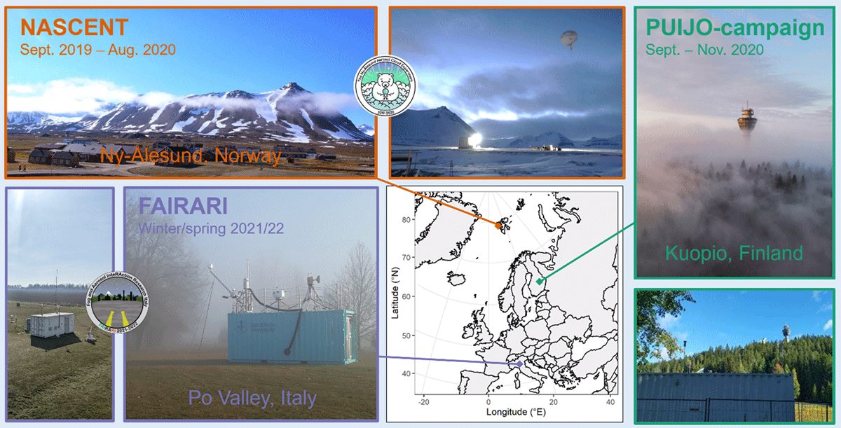
Figure 3
Overview of the in-situ measurement campaigns conducted within FORCeS: NASCENT in Ny-Ålesund, Norway, FAIRARI in Po Valley, Italy and PUIJO-campaign in Kuopio, Finland.
2.2.1 NASCENT
Observations during NASCENT (September 2019 to August 2020) were conducted at multiple sites close to Ny-Ålesund (78.9°N, 11.9°E). One of the key locations was the Zeppelin Observatory (485 m.a.s.l) located 2 km southwest of Ny-Ålesund on Mt. Zeppelin. Because of its location in a pristine Arctic environment, far from significant sources of contamination, interference from local pollution is minimal. Additionally, the prevailing meteorological conditions in the area further reduce the impact of local pollution. During NASCENT (from September 2019 to August 2020) the monthly cloud cover varied between 50% to 80% and from those 30 to 70% could be classified as low-level clouds. The measurements during NASCENT comprised a multitude of different variables to characterise the aerosols, clouds, radiation and meteorological conditions. Aerosol and cloud characteristics were observed with great detail, including e.g. the particle shape for the aerosols and both ice and liquid water content for the cloud measurements. Full details of the deployed instrumentation and measured parameters at each of the sites are given in Pasquier et al. (2022b).
2.2.2 PUIJO-campaign
The measurements during the PUIJO campaign (SMEAR IV station, 62.90°N, 27.65°E) included observations (from 15.09.2020 to 24.11.2020) at the top of the Puijo tower (306 m.a.s.l) and at ground level 200 metres below the tower station. The station represents a semi-urban environment, surrounded by forest and lakes but still resides in the vicinity (distance ~2 km) of Kuopio city centre. The site has been designed to investigate the interactions of aerosol particles and clouds, especially the activation of aerosol particles into cloud droplets. More details on the tower station can be found in Leskinen et al. (2009). The tower is frequently inside low-level clouds, and the ground station was used to obtain comparable observations for out-of-cloud conditions. At both stations, aerosol particle number size distribution and the chemical composition of the particles (dp < 1 µm) were measured. In the tower station, the particulate molecular composition was also measured along with droplet number concentrations and size distributions. Details of the measurements and instrumentation conducted during this campaign can be found from earlier work (Calderón et al., 2022; Kommula et al., 2024; Tiitta et al., 2022).
2.2.3 FAIRARI
The FAIRARI campaign took place at the research station San Pietro Capofiume in the Italian Po Valley (44.65°N, 11.62°E, 11 m.a.s.l) during winter/spring 2021/22 (with a pre-campaign in Feb 2021). The geography of the Po Valley, which is enclosed between the Alps in the North and West, and the Apennines in the South, promotes air stagnation under anticyclonic conditions. During winter, those, together with high concentrations of anthropogenic pollution (e.g. annual average PM2.5 > 25 µg m–3, Neuberger et al. 2025), often lead to long-lasting and dense fog events, affecting both visibility and human health. To evaluate the aerosol-fog interactions and their impact on secondary aerosol formation during this period as well as the transition to the following period of frequent new particle formation events, physical and chemical properties of gas molecules up to fog droplets were measured in situ. More details about the FAIRARI campaign, including a detailed description of the set-up, can be found in Neuberger et al. (2025).
3 Recommendations on Aerosol and Cloud Processes for Earth System Models
3.1 Recommendations for organic aerosol
Given the demonstrated structural uncertainties in the representation of OA impacts on the aerosol levels and ACI, with implications for, e.g. the representation of biogenic climate feedbacks (e.g. Blichner et al., 2024) and absorbing aerosol (e.g. Brown et al., 2021; Li et al., 2022b), it is evident that continued work on the representation of OA in ESMs is needed. The contribution of OA to the PNSD seems pertinent, as well as finding ways to simplify the complexity of the chemical system driving OA in terms of the number of simulated surrogate compounds and their assumed properties.
It is also evident that due to the large range of molecular species present in OA and the fact that many of them can change phase within the atmosphere, some form of treatment with various volatilities present in OA is needed. To address this issue, an ESM module called ORACLE-lite has been developed within FORCeS (Tsimpidi et al., 2025). Previously, the more detailed ORACLE module (Tsimpidi et al., 2014, 2018) was developed and implemented in the ECHAM/MESSy (Jöckel et al., 2006) Atmospheric Chemistry model EMAC (Sect. S1.3). ORACLE is based on the VBS approach (e.g. Donahue et al., 2006, see also Sect 1.1), uses fixed logarithmically-spaced saturation concentration bins and assumes the formation of pseudo-ideal solutions in the organic aerosol phase.
The overall aim of the ORACLE-lite is to combine advanced air quality features and recent experimental discoveries regarding the complexity of OA into a flexible, publicly available system. To meet the computational requirements for ESMs, the number of surrogate species describing OA and their volatility is reduced from 92 in ORACLE to 16 in ORACLE-lite (Figure 4). ORACLE-lite uses three surrogate species with effective saturation concentration at 298 K of C* = 10–2, 101, and 104 µg m–3 to represent the volatility range of low volatility (LVOCs), semi volatile (SVOCs), intermediate volatility organic compounds (IVOCs) emissions. These compounds are allowed to partition between the gas and aerosol phases, contributing to the formation of POA. Photochemical reactions that alter the volatility of gas-phase organic compounds are accounted for, and their oxidation products are tracked separately to simulate SOA formation from SVOC and IVOC emissions. Additionally, the oxidation of VOC precursors yields two products per species, distributed into two volatility bins with effective saturation concentrations of 1 and 103 µg m–3, which also partition into the aerosol phase and contribute to SOA formation. Overall, despite the simplifications applied to reduce the computational cost, ORACLE-lite is able to simulate the contribution of LVOCs, SVOCs, IVOCs and VOCs to OA formation with reasonable accuracy, underestimating total OA concentrations with normalised mean bias ranging from –4% over North America to –53% over Europe (Tsimpidi et al., 2025). Other existing ESMs could explore the implementation of ORACLE-lite, especially if their current simulations do not consider the variable volatility of organic species. The addition of 16 OA components comes at a computational cost and simpler approaches for OA representation could be desirable in some applications (Pai et al., 2020). In this regard, an evaluation of the ability of a given ESM to represent OA impacts on PNSD is encouraged—particularly, if capturing ACI is important for the model experiments in question. IOA species participate in NPF and early growth (e.g. Kupc et al., 2020), which implies the need for simulating the low-volatility components of OA. The approach developed and evaluated for EC-Earth-AerChem by Bergman et al. (2022) might therefore be of interest to models that seek a simple, yet thermodynamically-based representation of OA. This approach (noted as NEWSOA in Figure 5) focuses on two lumped species, namely semi-volatile and extremely low-volatile organic species (SVOCs and ELVOCs), results in generally improved predictions, though still underestimates aerosol number (Figure 5a) and optical depth (Figure 5b) compared with the earlier approach (noted as OLDSOA in Figure 5) in which SOA production was calculated offline (Bergman et al., 2022). Applicability of these recommendations naturally requires organic aerosol species to be represented in the model of interest, coupled to a gas-phase chemistry scheme and secondary aerosol formation processes.
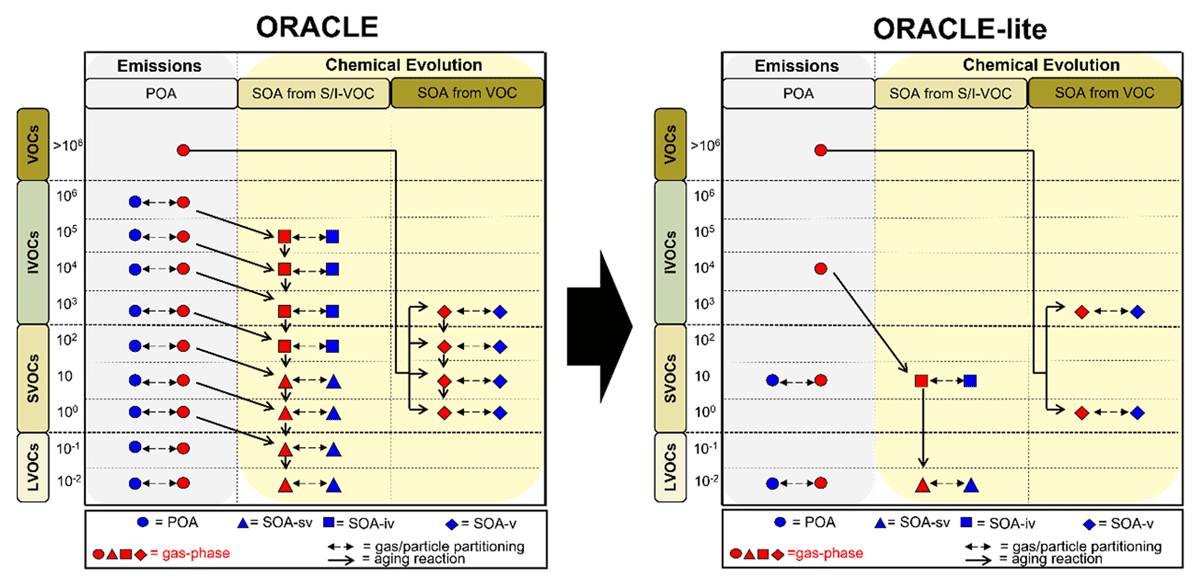
Figure 4
Schematic illustrating the difference between the full ORACLE (Tsimpidi et al., 2014, 2017) and ORACLE-Lite (Tsimpidi et al., 2025). Reproduced and modified under the Creative Commons 4.0 (CC 4.0) license.
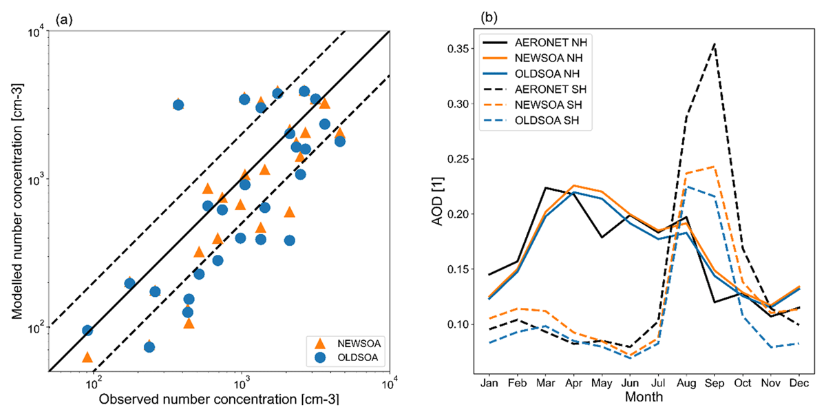
Figure 5
Evaluation of the performance between model simulations and observations presented in Bergman et al. (2022). Scatter plot in (a) shows the annual mean number concentrations at the stations (Table S3 in Bergman et al., 2022) in the year 2010, orange triangles indicate simulations with NEWSOA (online approach with lumped SVOCs and ELVOCs) and blue dots represent OLDSOA (offline calculation of SOA production). The black solid line shows the 1:1 line, and the dashed lines indicate a deviation of a factor of 2. Panel (b) shows the seasonal cycle of the mean AOD across all AERONET stations for Northern Hemisphere (NH, solid lines), and Southern Hemisphere (SH, dashed lines). Black lines indicate the derived AERONET AOD and the orange and blue colours are the NEWSOA and OLDSOA simulations, respectively. Figure adopted and modified from Bergman et al. (2022) under the Creative Commons 4.0 (CC 4.0) license.
As there are still large uncertainties in the volatilities of organics, Irfan et al. (2024) evaluated the sensitivity of globally simulated organic aerosol to the volatility of secondary organic aerosols. This study showed that although the growth of newly formed particles depends mainly on the organics with lowest volatilities, the simulated organic mass is most sensitive to semi-volatile organics due to the higher abundance of those species as well as the higher sensitivity to the partitioning process itself. Lowest volatility organics mainly reside in the particle phase, and this is not influenced by the small variability in their assumed volatility. Similarly, high volatility organics reside mainly in the gas phase and their partitioning is also insensitive to the variability in their volatility. Based on the same study, reducing the number of volatility classes by combining them requires a careful consideration of the mean volatility of the combined classes since the simulated organic mass and CCN are sensitive to these assumptions.
3.2 Recommendations for particulate nitrate
As anthropogenic SO2 emissions are decreasing, the importance of particulate nitrate will likely increase and ammonium nitrate is expected to surpass ammonium sulfate in the aerosol composition in many regions (Aksoyoglu et al., 2017; Tsimpidi et al., 2025; Wang et al., 2020). It is therefore recommended to review the treatment and consider the addition of nitrate within any ESM targeting on interactions between air quality and climate. We explored the key mechanisms driving nitrate formation on dust and sea-salt particles and evaluated how these processes are represented in models. By integrating different levels of complexity of the dust heterogeneous chemistry into the MONARCH model (see Sect. S2.2), we assessed the sensitivity of nitrate formation to various processes (Soussé Villa et al., 2025). The analysis focused on the condensation of gas species onto dust (both reversible and irreversible pathways), the impact of nitrate representation on species burdens, lifetimes, size distributions, and the role of dust alkalinity (mineral composition). Accounting for the alkalinity of dust and sea salt improved model agreement with observations, particularly when assuming reversible gas condensation onto dust particles and accounting for kinetic limitations. In contrast, irreversible uptake led to an overestimation of coarse particulate nitrate. As stated in Sect. 1.2 the main issue related to modelling inorganic aerosol thermodynamics in ESMs is related to the computational cost of these calculations. A computationally efficient atmospheric aerosol thermodynamics module, ISORROPIA-lite, has therefore been developed within FORCeS with the aim to be incorporated into ESMs with little additional computational cost. Special emphasis was placed on reducing the computational cost of the formation and evaporation of ammonium nitrate, the reactions of nitric acid with coarse sea salt and dust particles, and the competition between fine and coarse particles for the available nitric acid. The implementation of ISORROPIA-lite naturally becomes meaningful in models in which the key inorganic species described in the model are represented, together with a scheme aiming at predicting the thermodynamics of atmospheric water.
The ISORROPIA-lite module is described in detail by Kakavas, Pandis and Nenes (2022), and is based on the well-documented aerosol thermodynamics model ISORROPIA-II (see e.g. Fountoukis and Nenes, 2007). The main differences between the lite version and ISORROPIA-II are that it (1) assumes the aerosol is always in metastable (i.e. aqueous state) equilibrium, (2) treats the thermodynamics of Na+–NH4+–SO42––NO3––Cl––Ca2+–K+–Mg2+–Organics–H2O aerosols using binary activity coefficients from precalculated look-up tables, and (3) accounts for the contribution of organic aerosol water. The assumption of a metastable state greatly simplifies the phase diagrams, but is, however, supported by observations (Bougiatioti et al., 2016; Guo et al., 2015, 2018). The evaluation of ISORROPIA-lite compared to ISORROPIA-II within the chemical transport model PMCAMx (Sect. S2.1 and references therein), showed that the lite version is 35% faster accelerating the PMCAMx 3D simulations by ~10% (Kakavas, Pandis and Nenes, 2022). Further evaluation of ISORROPIA-lite in the EMAC (ECHAM5/MESSy, Sect. S1.3) atmospheric and chemistry-climate model compared to ISORROPIA II in stable mode showed relatively good agreement for global daily mean surface concentrations of inorganic aerosols, mineral ions and aerosol water (Milousis et al., 2024). Greater differences were found for intermediate humidity ranges (RH between 20% and 60%), where ISORROPIA-lite predicted higher aerosol water and lower particulate nitrate concentrations, due to the metastable assumption. The differences in particulate nitrate between the two versions were localised to specific regions, including the Middle East, the Himalayan Plateau and East Asia, with a strong dependence on RH. Meanwhile, the estimates from ISORROPIA-lite closely reproduced the AMS measurements of particulate nitrate, showing good overall agreement (Figure 6). While some scatter is evident, particularly in regions like North America, the model captures average nitrate concentrations well across regions, with normalised mean biases below 10% (Tsimpidi et al., 2025). This variability is typical of global models and originates from known limitations such as coarse spatial resolution and uncertainties in precursor emissions, as discussed in Milousis et al. (2025a).
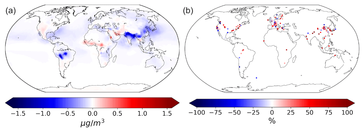
Figure 6
The change of the EMAC-simulated nitrate concentrations at surface after employing ISORROPIA-lite (vs. ISORROPIA II) is presented in (a), with blue colour indicating lower concentrations by ISORROPIA-lite. The coloured points in (b) show the deviations between EMAC results (with ISORROPIA-lite) and nitrate derived from observations with aerosol mass spectrometers around the world over the period 2000–2020.
Since the partitioning or semivolatile inorganic components is usually not simulated in ESMs and yet it might change under future conditions, our recommendation from FORCeS is to use a thermodynamic model within the ESM to perform these calculations if possible. This module could be, for example, the ISORROPIA-lite developed within FORCeS due to its reduced computational cost and good overall performance compared to the standard version of ISORROPIA-II (Figure 6a). Within FORCeS, the EQSAM module in EC-Earth3-AerChem has been replaced by ISORROPIA-II (Myriokefalitakis et al., 2022), in which nitrates are now simulated for both the accumulation and coarse mode, in contrast to the bulk aerosol approximation used earlier. Due to the good agreement between ISORROPIA-II and ISORROPIA-lite, a similar behaviour is expected with ISORROPIA-lite except for the reduced computational time.
Minerals present in dust, such as calcite, influence the aerosol pH and thus the distribution of nitrate between the gas and particulate phases (e.g. Karydis et al., 2021). However, deserts around the world have different mineral compositions due to their discrete soil characteristics, which can affect the coating of the emitted mineral dust with inorganic acids such as nitrate (Karydis et al., 2016; Klingmüller et al., 2018). ESMs typically assume a globally uniform dust chemical composition. Representing calcite in ESMs requires at least two additional tracers (for accumulation and coarse modes). This is now included in EC-Earth3-AerChem (Myriokefalitakis et al., 2022). Another potential option to avoid the extra computational cost is to use precalculated monthly climatologies of calcite fractions in dust. Within FORCeS, a new dust climatology has been developed that can allow ESMs broadly characterising regional changes in dust composition and its potential impact on aerosol pH and nitrate (Gonçalves Ageitos et al., 2023). In applications in which an accurate prediction of the distribution of nitrate between the fine and coarse mode is essential, our recommendation is therefore to consider implementing a dust minearology climatology (see also Sect. 3.3.2). These recommendations are meaningful additions for models that have dust represented as an aerosol species, coupled to some form of size-resolved composition (i.e., to separate between fine and coarse particles) and secondary aerosol formation.
3.3 Recommendations for absorbing aerosol
3.3.1 Black carbon
It is recommended that models align with the recent experimental determinations of fresh black carbon (BC) MAC at 500 nm by (Liu et al., 2020), who reviewed the available literature on BC absorption properties, and found an average of 8 ± 0.7 m2 g–1. This value is close to the MAC value of 7.5 ± 1.2 m2 g–1 recommended by Bond and Bergstrom (2006). Most of the numerical modelling studies align with this MAC recommendation, and use a refractive index of BC of 1.95 + 0.79i, which, however, according to Liu et al. (2020), can fail to reproduce the measured MAC values, resulting in a potential negative bias in the simulated BC absorbivity. Note that the recent AeroCom Phase III intercomparison exercise for absorbing aerosol by Sand et al. (2021) has reported that the BC MAC at 550 nm in 15 participating models ranged between 3.1 m2 g–1 and 16.6 m2 g–1, with a mean of 9.8 m2 g–1 and a median of 10 m2 g–1. However, not all models within the intercomparison provided values for BC MAC. While MAC values for aged (coated) BC larger than 10 m2 g–1 have been confirmed by several field observations, the values smaller than 7.5 m2 g–1 even for fresh uncoated (fresh or externally mixed) BC seem unsupported by the observations, and may require revision of the employed refractive index in the model.
In general, BC MAC is highly site-specific and can vary substantially, particularly in remote regions where aerosols are aged. This variability adds complexity, and sensitivities of models to updated MAC values are not yet fully known. MAC is also influenced by black carbon density, and the choice of the actual combination of values of density and refractive indexes can significantly impact the estimate of BC radiative forcing in global models (Digby et al., 2025). According to Liu et al. (2020), the density of black carbon aerosols is reasonably well constrained by laboratory measurements in the range 1.7–1.9 g cm–3. Nevertheless, the determination of black carbon density in ambient, internally mixed particles remains a topic of open investigation. Despite these uncertainties, MAC remains a powerful diagnostic of BC absorption and its evaluation in ESM output is highly recommended.
3.3.2 Dust
The direct influence of dust aerosols on climate is largely through their shortwave (SW) optical properties, which depend on mineral composition. ESMs often simplify dust as a single, homogeneous aerosol, ignoring regional differences in mineralogy. Studies have shown that variations in dust mineralogy, especially iron oxides like hematite that strongly absorb solar radiation, can significantly alter dust’s SW radiative effects (Li et al., 2021a; Perlwitz, Pérez García-Pando and Miller, 2015). We provide specific recommendations to improve dust mineralogy representation in ESMs, drawn from FORCeS investigations in collabaration with other projects like FRAGMENT and NASA EMIT (Earth Surface Mineral Dust Source Investigation) using the MONARCH model and other ESMs (CESM, NASA GISS ModelE and GFDL AM4) (Gonçalves Ageitos et al., 2023; Li et al., 2024a; Obiso et al., 2024; Song et al., 2024 and references therein). The focus of these recommendations is on levaraging new data (e.g. NASA’s EMIT mission surface mineralogy altas) and on refining iron oxide optical properties and mixing assumptions, while balancing accuracy with computational efficiency. These recommendations naturally become meaningful for models that simulate dust as an absorbing species.
The first recommendation is to move beyond globally uniform dust properties by allowing dust optical properties to vary geographically according to source mineral composition. Dust mineralogy differs by source region, which in turn affects optical behaviour. Yet many state-of-the-art ESMs still assume dust has invariant composition everywhere. Obiso et al. (2024) shows that by implementing individual tracers for key minerals and integrating region-specific soil mineral profiles from Claquin et al. (1999) into a model (with iron oxides as a key variable), the model produced higher SSA and thus a stronger cooling than the previous uniform-composition case, in substantially better agreement with dust-filtered SSA retrievals derived from AERONET (see also S5.2) sun photometers. Song et al. (2024) likewise found that explicitly resolving eight mineral types in the GFDL model reduced dust SW absorption compared to the homogeneous dust assumption, leading to better agreement with observations. The recommendation is to implement individual tracers for key minerals to spatially resolved dust composition in ESMs.
Underlying soil mineralogical atlases drive the modeled dust composition, so using the best available data is essential. Gonçalves Ageitos et al. (2023) examined two existing global soil mineralogy datasets (Claquin et al., 1999; Journet, Balkanski and Harrison, 2014) and found large discrepancies – for impactful components like iron oxides, different soil atlases led to 100% differences in the dust iron fraction in some regions. Such uncertainty directly translates to uncertainty in dust SW absorption in models as shown in (Li et al., 2021a, 2024a). Li et al. (2024a) likewise reported substantial bias in modeled hematite abundance when using current surface mineral datasets, underscoring the need for improved sources. The recommendation is to update model surface mineral inputs with new high-quality observations. The NASA EMIT mission offers a breakthrough dataset, using imaging spectroscopy to map surface mineral composition across major dust source regions (Clark et al., 2024; Green et al., 2023; Thompson et al., 2024). EMIT’s measurements can capture the spatial variability of minerals such as hematite with unprecedented detail. The first version of the new dataset has been implemented in four models (MONARCH, CESM, ModelE and AM4) to simulate the spatially and temporally varying refractive indices consistent with the varying mineralogical composition of dust aerosols, showing good agreement with SSA observations, and reduced uncertainty in the direct radiative impacts of dust in both present-day and future climates (Li et al., 2024b).
We furthermore recommend to update refractive indices for hematite and goethite, using improved optical constants for hematite and goethite based on recent laboratory constraints. Li et al. (2024a) and Obiso et al. (2024) highlight that hematite’s absorption capacity in dust has been highly uncertain (varying over two orders of magnitude) and substantially narrow this range by exploring mixing assumptions using lab measurements of dust composition, absorption, and scattering from Di Biagio et al. (2019) and mineralogy-aware dust modeling. Incorporating these refined properties in model radiative calculations reduced uncertainty in dust absorption. This ensures dust optical properties (like single-scattering albedo) are more realistically presented, directly improving estimates of dust’s direct radiative effect. In practice, ESM developers may replace older hematite optical parameters with the new values from Li et al. (2024a) or Obiso et al. (2024) based on Di Biagio et al. (2019) to better capture dust’s solar absorption. Model evaluation against observations (e.g. AERONET aerosol optical depth and single-scattering albedo) can confirm that this update leads to improved agreement. Since mineralogy also partly determines the desert surface albedo, updates to the dust composition will need to be accompanied by updates in the desert surface albedo to avoid biases in the dust direct forcing efficiency due inconsistencies between the optical properties of the dust and the desert surface.
Key minerals should be targeted, considering computational efficiency. We suggest focusing on representing those minerals that most strongly influence shortwave optics—primarily iron oxides (hematite/goethite)—for absorption. Other minerals such as calcite, feldspar and quartz may be of relevance when considering dust heterogeneous chemistry and the impact of dust on ice nucleation. All in all, modeling every individual mineral is impractical and computationally expensive, and the choice should depend on the application. Song et al. (2024) suggest grouping similar minerals to save computation: for example, treat all clay minerals (illite, kaolinite, smectite) as one category with shared optical properties, while keeping iron oxide-rich particles separate, since hematite and goethite have unique absorption characteristics. In their tests, lumping clays together and explicitly isolating hematite (and gypsum, another distinct mineral) maintained accuracy in radiative effects but with lower computational cost. Song et al. (2024) also found that a homogeneous dust tuned to a certain amount of hematite could mimic the global-mean radiative effect of a full mineralogy model. This implies that much of the climate impact comes from the overall dust absorption level. Thus, if computational resources are constrained, one minimum step is to adjust the assumed global dust iron oxide content together with the associated dust refractive index to observation-constrained values, to at least get the correct average SW absorption. However, for regional accuracy and mechanistic studies (e.g. impacts on monsoons), explicit spatial variation of mineralogy is preferable despite the extra computation. ESM developers should therefore represent at least the iron oxide fraction as a separate entity (or a separate optical property calculation), and possibly group the rest into a few broad classes (e.g. clays, quartz/feldspar, carbonates). An additional alternative is to use a globally resolved climatology of mineral fractions, representing some regional variability in dust optical properties, while avoiding the computational burden of additional mineral tracers. All in all, this balances detail with efficiency: the model gains realism in SW absorption by iron oxides without needing to track a dozen mineral tracers.
3.3.3 Brown carbon
Representing BrC in ESMs naturally requires OA to be explicitly parametrised, as BrC stands for the absorbing part of it. Only the absorption by BrC (i.e., the imaginary part of the refractive index) therefore has to be considered, while the scattering properties (real part of the refractive index) are considered through the OA direct climate effect. For a simple but explicit calculation of BrC, three different BrC species can be be considered: two primary strongly absorbing species and one photobleached very weakly absorbing species, denoted as pbBrC. The BrC produced during the oxidation of aromatic VOCs is weakly absorbing compared with the primary BrC and has rapidly decreasing absorbing properties due to ageing (Schnitzler et al., 2022). Thus, it could be neglected as a first approximation. The first primary BrC component to be considered is inert and insoluble and does not lose its absorbing properties, corresponding to 6–10% of BrC emissions (Forrister et al., 2015; Skyllakou et al., 2024). The second primary BrC component is soluble and loses its absorbing properties by photobleaching and is transformed to pbBrC. For this reaction, a rate constant k = 3.4 × 10⁻⁵ s–1 (Wong et al., 2019) or alternatively a rate depending on OH radical concentration (Wang et al., 2018) should be used. All BrC species to be considered are in the accumulation mode and are subject to atmospheric deposition. However, ongoing and future research is expected to clarify the key environmental factors that influence BrC photobleaching (Schnitzler et al., 2022) and regional patterns (Carter et al., 2021). These recommendations naturally require the OA scheme to be coupled to an atmospheric oxidation chemistry module.
For primary BrC, the imaginary part of the refractive index of BrC (kBrC,λ) is derived from the Mass Absorption Efficiency (MAE) and depends on wavelength. A value of 0.045 (MAE of 1 m2 g–1) is used for primary BrC at 550 nm and an Absorption Angstrom Exponent (AAE) of 5 for wavelength λ < 2 μm in the equations by (Zhang et al., 2020). Importantly, a particle density ρ of 1.3 g cm–3 is used for all BrC tracers in these recommendations. For the photobleached BrC at 550 nm, a MAE of 0.19 m2g–1, a kpbBrC of 10–3 and an AAE of 5 can be used within the range provided by (Saleh, 2020). Primary BrC sources to be considered result from biomass burning and biofuel combustion and can be calculated (as mass equivalent to absorption) in two ways: either using the BC/OA emission ratio (see Zhang et al., 2020), or as associated to the ELVOC species in the model (Skyllakou et al., 2024; Tasoglou et al., 2020). The second approach is found to lead to about 10 times lower BrC emissions from biomass burning over Europe (Skyllakou et al., 2024), pointing to the need to further improve the emissions of BrC from its various sources through targeted field and laboratory studies.
The OA effective absorptivity at 550 nm (AOA,550) and the equivalent mass emissions of BrC have been parameterised by Zhang et al. (2020) as a function of the BC to OA emission ratio by (Saleh et al., 2014) based on multiple laboratory experiments on fresh and aged BrC emissions, and using source-specific emission rates of OA, BC and BrC (EOA, EBC, EBrC, respectively) in g m–2 s–1. Figure 7a shows the global AAOD at 440 nm of BrC in TM5 (the atmospheric chemistry and aerosol model component of EC-Earth3-AerChem). As the aerosols are internally mixed in the model, BrC AAOD for Figure 7a was extracted by running two separate simulations; one without BrC and with OA being only scattering (imaginary part of the refractive index being zero), and the other as described above. The difference between these two simulations in the total AAOD was then taken to obtain the AAOD for BrC. It is clear that AAOD maxima appear in central Africa, India and Eastern China, and high values over the Amazon, which are areas affected by biomass burning events.
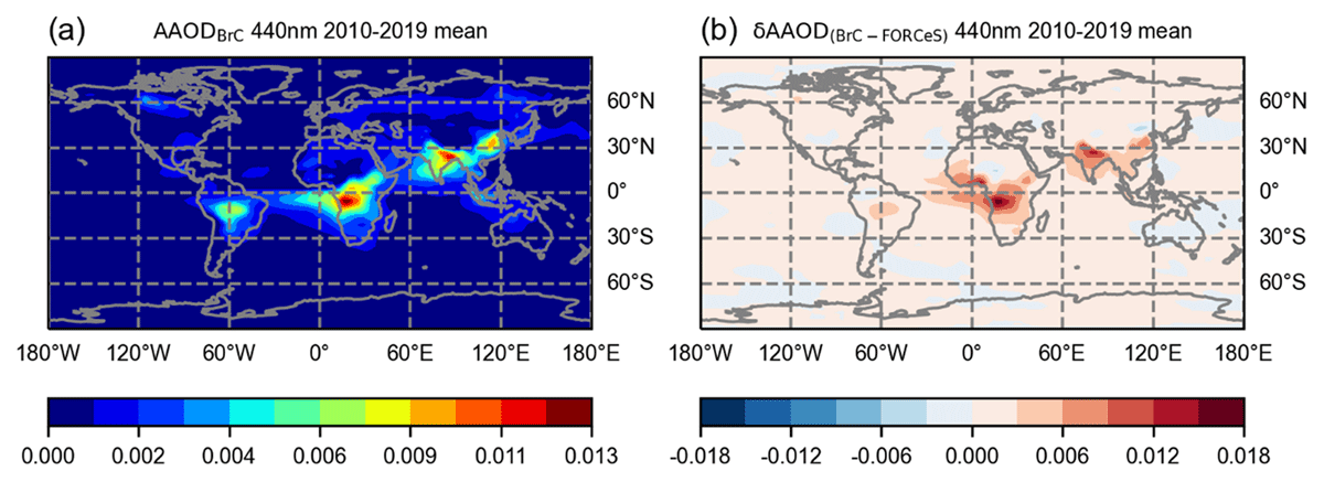
Figure 7
Absorption Aerosol Optical Depth (AAOD) for BrC at 440 nm is presented in (a). AAOD for BrC is calculated by the difference between two ten-year simulations, one accounting for BrC and the second one neglecting its absorption. In (b), the difference in AAOD at 440 nm between a simulation in which all OA is considered slightly absorbing (referred to as FORCeS) and a simulation where OA are only considered scattering and BrC only absorbing (referred to as BrC). Both subfigures display averages over ten-year periods (2010–2019).
In Figure 7b, the difference in BrC AAOD at 440 nm is shown between a simulation in which all OA are considered slightly absorbing (referred to as FORCeS) and a simulation that accounts for both only scaterring OA, i.e. the imaginary part of the refractive index is set to zero, and only absorbing BrC, i.e. the real part of refractive index is set to one. This simulation is referred as BrC in Figure 7b. The latter—i.e. the BrC simulation—shows higher AAOD over biomass-burning affected areas, and slightly lower AAOD at remote areas where in the FORCeS simulation OA was slightly absorbing. These results demonstrate the importance of individual consideration of BrC absorption in climate models.
An evaluation of BrC absorption, simulated by the MONARCH atmospheric chemistry model adopting the parametrisation described above, showed reasonably good correlations with aethalometer observations across Europe (Navarro-Barboza et al., 2025). However, despite accounting for primary biomass burning and biofuel sources, the simulated BrC absorption was still notably underestimated at the sites analysed. These underestimations could be attributed to unaccounted or underrepresented sources, highlighting the need for further studies to derive refined anthropogenic BrC emission inventories (Xiong et al., 2022).
3.4 Recommendations for new particle formation and ultrafine aerosol
Numerous global and regional scale modelling studies have demonstrated that the formation of new secondary aerosol particles through NPF is a key process modifying the aerosol PNSD and CCN concentrations, and hence should be accounted for in some way within any ESM that aims to investigate ACI (Dunne et al., 2016; Stolzenburg et al., 2023; Zhao et al., 2024). The representation of NPF within ESMs can, on the one hand, rely on (essentially semi-empirical) parametrisations of field observations, or on the other hand on laboratory observations of NPF involving known chemical systems, or some kind of combination thereof. Balancing the need to reproduce present particle number concentrations with a reasonable accuracy with the need for mechanistic parameterisations with maximal predicting power in different environments and conditions requires following both of these development tracks in parallel. Besides the chemical systems considered for NPF within models, the size range into which new particles are added also varies, depending on the PNSD description and NPF schemes used within the model. Again, extending the PNSD description to the sizes that allow for a more mechanistic description of NPF instead of saving computation resources for more important processes is a delicate balancing act. However, recent studies demonstrate the ability of Aitken mode particles with diameters well below 50 nm to contribute to CCN concentrations (e.g. Bulatovic et al., 2021; Karlsson et al., 2021), particularly in clean environments (see also Sect. 3.5). To capture ACI, a PNSD representation is of importance, including the key processes modifying the Aitken mode (including the contribution of NPF to particle number within it). For the applicability of recommendations related to NPF, it is therefore important to ensure that Aitken mode dynamics are also represented within ESMs, Blichner et al. (2021) implemented a sectional scheme for the smallest particles (5–39.6 nm diameter) in NorESM2. This improved the concentrations of the smaller particles (50 nm < dp < 100 nm) compared with observations. In addition, this led to an increased concentration of cloud droplets in remote regions, implying that an inadequate representation of the smallest aerosols can indeed have considerable impacts on the predicted aerosol-cloud interactions.
Within FORCeS, we have investigated the observed atmospheric formation rates (J) of particles in different environments (Figure 8a): boreal forests (the SMEAR I and II stations in Hyytiälä and Värriö in Finland), urban areas (Beijing, China and Budapest, Hungary) and rural sites (Agia Marina Xyliatou in Cyprus and Maracapuru in Brazil). Using data from such different environments hopefully allows the creation of parametrisations that are simple yet applicable in various environments globally (Li et al., 2025). Based on these observations, the formation rate of 5–9 nm particles (J5) was parametrised by using RH, observed sulfuric acid concentration (H2SO4) and condensation sink (CS) as input variables – these are also then needed for the applicability of the parameterisation. The obtained equation can be expressed as
where k0 = 1490.02, kSA = 0.23, kRH = –2.53 and kCS = 0.67 are the experimentally derived coefficients (Li et al., 2025). It is known that various oxidation products of VOCs, highly oxygenated molecules (HOM), also participate in the first steps of new particle formation and growth (see Sect. 3.1). Despite the insufficient long-term VOC data, sulfuric acid is assumed to be the main vapour for the purpose of this parametrisation due to its global abundance. The developed parametrisation for J5 has been preliminary evaluated with the TM5 module (employed, for example, in EC-Earth3-AerChem). The results (Figure 8b, blue line) show that the underestimation of Aitken mode aerosols is fixed with the new parametrisation compared to the simulation without nucleation (orange line). This parametrisation, presented in Eq. (1), can therefore be recommended if a field-based semi-empirical approach is desired.
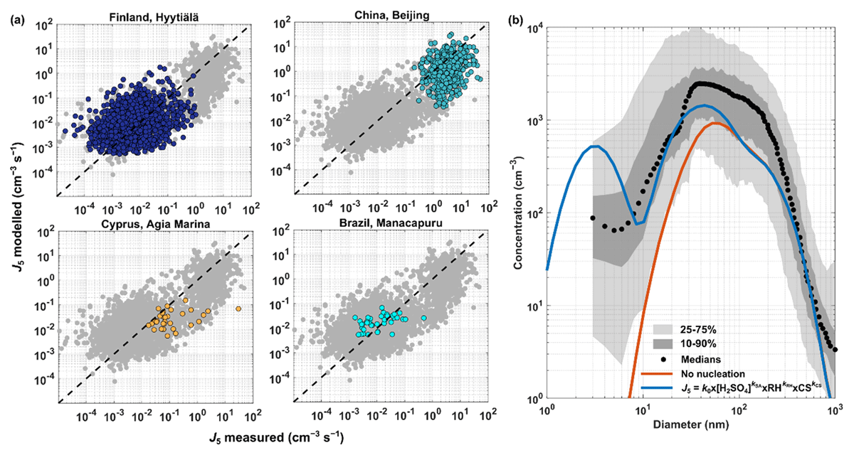
Figure 8
Preliminary J5 parametrisation testing results on several environment types involving boreal forests, giga-city, rural and rural/rain forest zone is shown in (a). Coloured points refer to the measurements at the specific sites and grey points show all measured data as presented in Li et al. (2025). The dashed lines are 1:1 line for the comparison between the measured and the modelled J5 values. In (b), TM5 simulation results for particle number concentration using Eq. (1) are shown as 2018 December medians (black dots and their shades) from pristine boreal forest, arctic remote boreal forest, urban, and rural regions as tests. “No nucleation” refers to no applied nucleation mechanism in TM5 simulation, and Eq. (1) showed promising prediction power, especially for particles at CCN size.
A complementary approach to using field observations for parametrising NPF is to use well-controlled laboratory observations of known chemical systems, and to sum up these NPF parametrisations within a potential ESM application (see e.g. Dunne et al., 2016; Zhao et al., 2024 for examples). The CLOUD chamber (Sect. S4.1) is one of the most important laboratory facilities used at present to investigate NPF, and the chemical systems studied by CLOUD up to the end of 2022 have been summarised in a recent review by Kirkby et al. (2023). These systems include those involving sulfuric, nitric and iodic acids, water, ammonia, various amines, as well as some biogenic and anthropogenic organic species. In general, the NPF studies from CLOUD report particle formation rates (J) at the low-end of the particle number size distribution measurements, usually around 2 nm, as a function of the concentrations of the relevant nucleating vapours—most importantly sulfuric acid, the least volatile oxidation products on the organic precursors, or iodic acid. In many of the studies reviewed within Kirkby et al. (2023) these laboratory observations have then been cast into simplified parametrisations (Dunne et al., 2016; Gordon et al., 2016; Lehtipalo et al., 2018), that can be utilised within larger-scale models, including ESMs (see also Zhao et al., 2024). A complementary, less empirical, method with great potential in reproducing observed NPF and its impacts of ambient PNSD uses look-up tables or other simplifications of predictions from kinetic cluster models (McGrath et al., 2012) with the cluster energetics constrained by laboratory observations (e.g. Roldin et al., 2019) instead of essentially semi-empirical fits. Additional work conducted in the SAPHIR* chamber (Sect. S4.2) has shown, for example, that shifting chemical regimes from RO2 dominated to HO2 and NO dominated has a clear effect on HOM product distribution, thus also having impact on the SOA yields (Baker et al., 2024).
The issues that remain to be specified in any respective ESM application are therefore 1) which gas phase species to involve in the NPF parametrisation (based on the which tracers are simulated in the model); 2) which size range the particles are (based on the PNSD representation present in the model); and 3) how the condensation growth and coagulation of these new particles are treated (based on both, see e.g. Stolzenburg et al. (2023) for a review on nanoparticle growth, including its representation and effects within ESM applications).
Observational and theoretical studies (Bardakov et al., 2024; Brock et al., 1995; Curtius et al., 2024; Kupc et al., 2020; Weigel et al., 2011; Williamson et al., 2019) have shown that besides NPF taking place in the atmospheric boundary layer (BL), some of the CCN might have actually originated from NPF at higher altitudes (i.e. upper troposphere, UT) and are transported downwards within the atmosphere. However, NPF in the UT is limited to whether the necessary precursors can be transported to the UT in the required quantities. Wang et al. (2022) for example, demonstrated the possibility of intense synergistic nucleation of HNO3, H2SO4 and NH3 (available in necessary amounts) in the UT. Nucleation of organic species in the UT is also an important mechanism contributing to aerosol abundances in the UT. Of all organic species, especially isoprene and monoterpenes are the most important reactive organic species emitted by plants in the tropics. In addition to contributing to the growth of newly formed particles, they can also directly contribute to particle formation in combination with other species (see e.g. Ehn et al., 2014; Kirkby et al., 2016; Lehtipalo et al., 2018; Riccobono et al., 2014; Tröstl et al., 2016) or nucleate on its own (e.g. Simon et al., 2020). Palmer et al. (2022) linked overnight convective transport of isoprene to large amounts of tropospheric aerosols later in the day. Particle nucleation from isoprene was subsequently confirmed and analysed in detail by (Bardakov et al., 2024; Curtius et al., 2024; Shen et al., 2024). While the nucleation processes itself can, in principle, be captured with the same particle formation rate parametrisations as NPF within the BL, a proper understanding of aerosol precursor loss and chemical transformation during cycles of deep convection is essential (see also Sect. 3.8.3) to accurately predict aerosol, and further CCN abundances in the UT. Given the recent knowledge accumulated on the potential role of multiple different chemical systems capable of nucleating new particles in the Earth’s atmosphere, the applicability of the laboratory-based parameterisations mentioned above depends on the comprehensiveness of the chemical systems required. Representing all potentially nucleating species explicitly in ESMs is probably not cost-effective given present computational resources and other priorities, hence there is a continued need for reconciling the insights from laboratory studies with field observations, and developing simple yet general schemes for new generations of NPF parameterisations with improved predictive power.
3.5 Recommendations for droplet activation and droplet concentration susceptibility
3.5.1 Cloud droplet activation
On a principal level, the recipe for predicting the activation of aerosol particles to cloud droplets is relatively well established: if the particle number size distribution, chemical composition and ambient water vapour supersaturation is known, the fraction of particles that can grow into cloud droplets can be rather accurately predicted using the Köhler theory (Calderón et al., 2022; Köhler, 1936). In the atmospheric context, the supersaturation is often driven by cooling caused by several small-scale processes such as buoyancy, orographic effects, radiation or atmospheric mixing.
A comprehensive review of the numerous available droplet parameterisations was performed by Ghan et al. (2011). They found that the more complex iterative-based schemes, such as the one from Fountoukis and Nenes (2005), performed well when compared against an adiabatic cloud parcel model under a wider range of environmental conditions, and usually performed better when compared to the non-iterative schemes. In the non-interactive schemes, more Nact was estimated for higher aerosol concentrations, and lower Nact for low aerosol concentrations, compared to the iterative scheme from Fountoukis and Nenes (2005).
The study of Simpson et al. (2014) performed an evaluation against a cloud parcel model of the Abdul-Razzak and Ghan (2000) and Fountoukis and Nenes (2005) schemes and its subsequent updates (Barahona et al., 2010; Morales Betancourt and Nenes, 2014) which include updates to account for the growth of inertially limited particles, and their subsequent contribution to the water vapour sink. They found that all these schemes tended to underestimate the fraction of activated drops compared to the parcel model due to the methods used by the parametrisations to approximate the sink of water vapour. Furthermore, Simpson, Connolly and McFiggans (2014) highlighteded a tendency of the parameterisations to overestimate the fraction of activated aerosol particles for simulations in which the aerosol particle median diameter of a single lognormal mode is large (between 250 and 2000 nm). They attributed this overestimation to the parametrisations having an infinite “effective simulation time” compared to the simulation time prescribed in the parcel model due to the assumption in parametrisations that the parcel rises to the altitude of Smax, regardless of whether this is greater than cloud top (Simpson, Connolly and McFiggans, 2014). This characteristic of existing droplet activation schemes requires further study, and should be considered carefully, for example, in future GCM simulations of geoengineering experiments such as marine cloud brightening.
A recent study found the performance of the Abdul-Razzak and Ghan (2000) scheme against a cloud parcel model to be sensitive to the geometric standard deviations (widths) of the lognormal aerosol modes (Ghosh et al., 2025). By adjusting three constant parameters within this scheme they were able to improve the performance of the parametrisation under polluted aerosol conditions. They compared both the original and modified Abdul-Razzak and Ghan (2000) scheme and the population splitting scheme of Morales Betancourt and Nenes (2014) against a cloud parcel model and found that the original Abdul-Razzak and Ghan (2000) scheme tended to underpredict Smax for almost all environmental conditions explored. The more complex scheme (Morales Betancourt and Nenes, 2014) was found to be in generally good agreement with the parcel model for all input parameters explored with similar agreement found from the updated Abdul-Razzak and Ghan (2000) scheme.
In summary, considering the importance of constraining GCM ACI forcing estimates which are strongly dependant on the accurate calculation of Nact in the present day, and during cleaner aerosol conditions during the pre-industrial period (Carslaw et al., 2013) it is recommended that GCMs and ESMs embrace the complex iterative based droplet activation parametrisation of Morales Betancourt and Nenes (2014) or the recently updated version (Ghosh et al., 2025) of Abdul-Razzak and Ghan (2000). It is also recommended that future development and evaluation of these parametrisations be undertaken against an ensemble of detailed cloud parcel models in a consistent way (e.g. Shipway and Hill, 2012), given that the reported performance will depend on differences in the numerical cloud models used to develop the original schemes. Additionally, the warm bias in sea surface temperature over the Southern Oceans simulated by the CMIP6 models has been a persistent issue (see Sect. 1.2). This bias is mainly attributed to the deficiencies in cloud processes, such as the lack of supercooled liquid water clouds resulting in insufficient reflection of SW radiation, exacerbating the warm bias. Recently, updates in the IFS cloud scheme (employed in EC-Earth-AerChem), including employment of the Morales and Nenes activation scheme, have been applied and shown to reduce this bias. For example, the work by Thomas et al. (2024) quantified the impact on biases in the cloud radiative effects, and observed reduction of approximately 40–50% over the Southern Oceans.
An important aspect to consider is the relative role of PNSD and OA hygroscopicity in governing ACI in ESMs. While PNSD typically dominates CCN activation by controlling the number of particles that can activate, hygroscopicity and mixing state provide crucial secondary influences, particularly in organic-rich or biomass-burning environments. Eventually, accurate representation of both factors is essential for reliable ACI estimates (Mandariya et al., 2024; Pöhlker et al., 2023; Shen et al., 2025; Xu et al., 2021b). In ESMs, their relative importance depends on the CCN activation parameterisation—simplified schemes could overemphasise PNSD effects, whereas those incorporating size-dependent chemistry or κ-based activation could, in theory, capture the coupled microphysical and chemical controls more realistically.
3.5.2 Susceptibility of cloud droplet number concentration to aerosol perturbations
Examining the relationship between the aerosol particle concentration (for different lower cut-off diameters) and the CDNC from long-term in-situ observations, remote sensing data, and ESMs reveals an important trend. The susceptibility of CDNC to perturbations in aerosol particle concentrations derived from ground-based in-situ observations is considerably higher than the corresponding response inferred from global ocean satellite data (Virtanen et al., 2025). Furthermore, the analysis reveals significant issues in how this process is currently represented within ESMs, calling for further work on this key driver behind ACI predictions. The data show that the typical critical activation diameter at Puijo (located in Kuopio, Finland) is around 125 nm, around 110 nm in Pallas (located in northern Finland), and as small as 40 nm for Zeppelin in the Arctic (Bulatovic et al., 2021; Karlsson et al., 2021). The findings support previous observational studies by Kecorius et al. (2019), Koike et al. (2019) and Willis et al. (2016), which indicate that Aitken mode aerosol particles are important for cloud droplet formation in clean environments. Parcel model calculations suggest activation diameters as small as 30 nm for some arctic conditions (Motos et al., 2023). The small activation diameters in the Arctic could also be linked to high contribution of marine sulfate to the total aerosol mass, especially during summer (Gramlich et al., 2023; Siegel et al., 2023).
High-resolution modelling (see also Sect. S3) work by FORCeS members also shows that Aitken mode particles significantly affect cloud microphysical and radiative properties in the summertime high Arctic when accumulation mode number concentrations are low (<10–20 cm3, Bulatovic et al., 2021). The modelling results obtained during FORCeS agree with observations of the Hoppel minimum obtained from multiple expeditions in the high Arctic (Bulatovic et al., 2021 and references therein). The results show that accumulation mode particles should not be considered as the only potential CCN in models, as this may lead to inaccuracies in CCN concentrations and their sensitivity to perturbations in various emissions. Even more subtle effects were observed in the Po Valley fogs (see also Sect. 2.2.3), where activation diameters are as large as 300–400 nm (Gilardoni et al., 2014), and aerosol number concentrations are in great excess with respect to the potential CDNC. Based on ongoing research, the actual supersaturation reached during activation and the number of activated droplets is first affected by the dispersion in the accumulation mode size distribution and secondly by the chemical composition. In aerosol-fog interactions in polluted environments, as a typology of an “updraft-limited regime” (Reutter et al., 2009), a realistic representation of the standard deviation of the accumulation-mode size distribution along with an at least synthetic formulation of aerosol hygroscopicity are therefore recommended.
The process-based evaluation of the ESMs by Virtanen et al. (2025) reveals that further development work is required on how the driving force for water vapour supersaturation—in practice the parametrisation of the cloud-scale updraft velocity—is represented in the models. The results from the three field sites presented in Virtanen et al. (2025) are generally in line with the findings from a review article led by and involving FORCeS partners, which pointed out the general need to improve satellite-based methods to derive aerosol-cloud relationships (Quaas et al., 2020). Combining constraints from satellite data, in-situ observations and high-resolution modelling show promise in providing further insights into cloud droplet activation processes. Taken together, the analysis conducted within FORCeS shows that, despite the fact that the fundamental microscale thermodynamics of cloud droplet activation are in most cases well understood (see, however, also e.g. Heikkinen et al., 2024; Lowe et al., 2019), the inputs (particularly PNSD and cloud-scale updraft velocity) required for the common parametrisations are not yet well enough constrained within current ESMs to provide an entirely consistent and robust representation of susceptibility and hence ACI (Virtanen et al., 2025). Furthermore, care must be taken when inferring the susceptibility of clouds to aerosol perturbations from remote sensing observations, as the potential link between aerosol products derived from remote sensing data and CCN concentration is not always straightforward (see also e.g. Jia et al., 2022; Manshausen et al., 2022), and the observations at the cloud top do not necessarily represent the condition at the cloud base where activation takes place. It is also important to note that perturbation of the local background aerosol conditions has different impacts in different environments (Kommula et al., 2024).
Additional work using the above mentioned LES modelling to develop ESM parametrisations was also conducted within FORCeS. ESMs and other large-scale models rely mainly on parameterising the subgrid component of the updraft velocity based on turbulent kinetic energy. In FORCeS, we have used an ensemble of marine stratocumulus clouds simulated with a large eddy model to develop a parametrisation that can be used to estimate the updrafts driven by radiative cooling (Ahola et al., 2022). The use of the new parametrisation in ECHAM shows that the method is a promising candidate and should be extended to cover other cloud types (Nordling et al., 2024). However, the work conducted within FORCeS also points out that the time step limitations on LES modelling can lead to overestimation of the susceptibility at very high aerosol concentrations or low updraughts in warm stratocumulus clouds (Schwarz et al., 2024).
3.6 Recommendations related to cloud microphysical processes beyond activation
As mentioned in Sect. 1.6, most current ESMs form precipitation through some form of autoconversion parametrisation (see e.g. Khairoutdinov and Kogan, 2000; Sundqvist, 1978). The work conducted within FORCeS (Prank et al., 2022, 2025) supports previous studies (Jensen and Lee, 2008; Jensen and Nugent, 2017) on the importance of considering coarse mode aerosol particles and giant CCN in the representation of autoconversion for capturing this process correctly. This update will most likely act to substantially modulate the timing of the drizzle onset in shallow cumulus clouds. The stratiform cloud cases are expected to show similar or possibly even stronger signal, which has substantial repercussions for the description of marine clouds in global models. For example, current methods are very likely to produce a delayed onset of drizzle in subtropical stratocumulus outflow regions near the coasts (see e.g., Magaritz-Ronen, Pinsky and Khain, 2016), where droplet concentrations are typically too high for drizzle initiation when autoconversion schemes neglect the presence of giant sea-salt particles. In these clouds, drizzle and precipitation formation can lead to reorganisation of the mesoscale cloud structure, transforming the cloud deck from a closed to an open cellular structure and causing dramatic changes in the overall albedo (e.g., Stevens et al., 2005). Accounting these particles is therefore critical for describing the aerosol-cloud interactions and the aerosol indirect effect. As contemporary climate models usually carry at least some information about the aerosol size distribution, it is therefore recommended that coarse mode aerosol is accounted for in the autoconversion parametrisation. Before the onset of autoconversion, the large end of the droplet size distribution is affected by sedimentation fluxes (as evident also in fogs, see e.g. Boutle et al., 2022). Additionally, given the high subgrid-scale variability of the processes and variables relevant for cloud microphysics, further work in the development of the ESM resolution is warranted.
Fogs can be considered as special cases of clouds that are in contact with the Earth surface. However, compared to other clouds, the growth in liquid water content is strongly controlled by the sedimentation of cloud droplets. As sedimentation becomes efficient already for droplets that are smaller than those typically formed from the autoconversion process, and thus the employment of autoconversion can lead to too efficient water removal. This is demonstrated in Figure 9, which visualises the evolution of radiation fog simulated with UCLALES-SALSA (Sect. S3.1): the droplets do not have time to grow to drizzling sizes (dp~100 µm, Figure 9c) before they are removed due to sedimentation. This is the case especially if the fog does not reach altitudes higher than 100 m, after which both droplet concentration (Figure 9a) and liquid water content (Figure 9b) reach high values due to the change in fog dynamics (Boutle et al., 2018). Our recommendation is to not use the autoconversion process at all when simulating fog, especially if the fog droplet formation is based on physically valid parametrisations that account for radiative cooling at the top of and activation processes within the fog. This recommendation is, however, most relevant for high-resolution models, as present ESMs do not generally have high enough resolution to explicitly simulate fog, although low-level clouds are common. Also, the assumption of the droplet size distribution shape in bulk models is affecting the water removal and thus liquid water content strongly (Boutle et al., 2022), and it is recommended that the bulk schemes should be evaluated against observation such as those performed during the FAIRARI campaign.
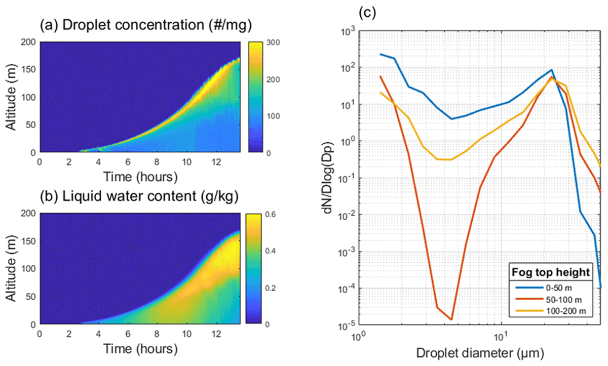
Figure 9
Example of the evolution of radiation fog. (a) droplet number concentration, (b) liquid water content, and (c) average fog droplet size distribution for the lowest 15 m during three different fog periods according to the fog top height. Simulations are conducted with UCLALES-SALSA (Sect. S3.1) in 2D setup employing the mean aerosol size distribution from the FAIRARI campaign (Sect. 2.2.3) and assuming constant aerosol hygroscopicity of 0.6. Vertical and horizontal resolution in the simulations were 1.5 m and 4 m. Atmospheric background sounding for initial conditions is typical for the nighttime radiation fogs observed in the area.
To include the effect of entrainment (see Sect. 1.6) there are two necessary ingredients: 1) Turbulence at cloud top needs to be a function of cloud-top radiative and evaporative cooling; and 2) cloud droplet sedimentation has to be a function of cloud droplet number/size, and has to be accounted for in the first place. Point (1) is to some extent fulfilled in all turbulence parametrisations directly or indirectly (via cooling rates). It is, however, not clear whether the effect is realistic enough. One of the potential problems is the lack of inversion strength and sharpness, due to the coarse vertical resolution (e.g. Pelucchi, Neubauer and Lohmann, 2021). The other problem is that not only turbulence, but also numerical diffusion leads to mixing and entrainment. It is only the former that is responsive to the aerosol-induced perturbation; the latter should be as small and irrelevant as possible. Point (2) is accounted for in several cloud microphysical schemes, but in many others it is not. The ones that consider cloud droplet sedimentation include the schemes by Morrison and Gettelman (2008) (see also Gettelman and Morrison, 2015; Seifert and Beheng, 2006).
The effect of mixing and evaporation on the impact of enhanced CDNC on cloud liquid water path and cloud fraction should be examined using observations. This should involve a statistical analysis as well as an analysis of the response of clouds to external perturbations. If ESMs simulate a reduction in LWP due to enhanced entrainment that is not large enough compared to observations, or if it is even overwhelmed by a positive LWP response, the first aim would be to reduce the impact of drizzle formation rather than attempting to directly increase the effect of entrainment. The results from FORCeS suggest that great care should be taken when inferring LWP responses to aerosol from remote sensing data. Arola et al. (2022) showed that the propagation of natural spatial variability and errors in satellite retrievals of cloud optical depth and cloud effective radius strongly impact estimates of aerosol indirect effects. They used satellite and synthetic measurements to demonstrate that, because of this propagation, even a positive LWP adjustment to an aerosol increase is likely to be misinterpreted as negative. This biasing effect would likely result in an underestimate of the aerosol-cloud-climate cooling. Similarly, Zipfel et al. (2022, 2024) showed that the relationship is modulated by precipitation fraction and sea-surface temperature, and that the sensitivity of LWP to CDNC is weaker at higher CDNC, based on a machine-learning approach. These conclusions were supported by a study from Kokkola et al. (2025) in which model outputs from UCLALES-SALSA (Sect. S3.1) for stratiform clouds were analysed using satellite retrieval equations. Similarly to the Arola et al. (2022) analysis, satellite retrieval equations biased the correlation between CDNC and LWP negative at higher CDNC values. However, this study indicated that, by carefully selecting cloud cases with similar meteorological conditions, and ensuring that cloud condensation nuclei concentrations are well-defined, changes in liquid water can be reliably determined using satellite data. Such data would also be useful for evaluating the description of LWP response to aerosol in ESMs.
Christensen et al. (2022) reviewed available satellite datasets and field campaigns to find opportunistic experiments of aerosol influence on cloud microphysics. Based on the satellite data analysis, they found that cloud albedo perturbations were strongly sensitive to background meteorological conditions and that LWP increases due to aerosol perturbations could generally not be distinguished from the data (in line with Arola et al., 2022). While they found these opportunistic experiments to give significantly improved process-level understanding of ACI, they also concluded that it remains unclear if the relationships found can be reliably scaled to the global level. Manshausen et al. (2022), on the other hand, took a closer look at ship tracks, leveraging from the fact that only a small fraction of the clouds polluted by shipping show ship tracks in satellite images. They showed aerosols emissions led to substantial changes in cloud properties even when no ship tracks were visible in satellite images. The study by Manshausen et al. (2022) indicated selection biases in previous studies of ship tracks, and found a strong LWP response to clouds to aerosols perturbations, which in turn potentially indicates a higher climate sensitivity than observed temperature trends would otherwise suggest (see also Watson-Parris et al., 2022, which discusses the importance of shipping regulations for climate). Machine learning approaches were also exploited within FORCeS in the investigation of cloud microphysical properties. Bender et al. (2024) found, for example, that the cloud droplet effective radius can be successfully estimated by gradient boosting regression using only meteorological data as input, and limited improvement in model skill with inclusion of aerosol information. The work highlights the importance of local meteorology on controlling cloud properties. Similarly, Jia et al. (2024) used explainable machine learning to quantify cloud-fraction adjustments to aerosol in the context of meteorological conditions. Proske et al. (2024) tested a drastically simplified approach and replaced the aerosol model in ECHAM-HAM with a CCN and INP climatology, as input for either of the two available aerosol activation schemes (Abdul-Razzak et al., 1998; Abdul-Razzak and Ghan, 2000 or Lin and Leaitch, 1997). The simplification reduced the computational time up to ~65%, while deviations in results from the simplified model stayed mostly close to inter-annual variability of the full model version. Depending on the purpose of a modeling project, a simplified model version may indeed be more apt than a complex one. In particular, the work from Proske et al. (2024) highlights the role of simplification for understanding: it generates an easier-to-understand model version, but also creates understanding through the simplification work itself.
An important aspect of model evaluation is to determine the extent to which the model is simultaneously consistent with multiple observation types. A model that is skilful at simulating one aerosol or cloud property (e.g., droplet number concentration) but inconsistent with another (e.g. aerosol optical depth) or vice versa is not a realistic model. In normal global model development in which adjustments to parameter values are usually made one at a time, such “cross-variable consistency” is difficult to establish because not all potential combinations of parameter values are explored (i.e. retuning could eliminate cross-variable inconsistency). In FORCeS, a new approach was developed that exploited a perturbed parameter ensemble to detect such cross-variable inconsistency by examining model-observation skill across 37-dimensional space of uncertain parameter combinations in UKESM1 (Regayre et al., 2023). In this study, one million model ‘variants’ were created using emulators trained on UKESM1 (Sect. S1.1) simulations and were then evaluated against observations of several cloud properties in several ocean regions and months of the year (in total 450 observational constraint variables). The study then constrained to each of these observation variables separately and quantified the effect on the model-observation agreement with the other variables. This approach exposed a very large number of pair-wise inconsistencies that indicate potential structural deficiencies in UKESM1 – i.e. achieving model consistency with two variables simultaneously would require changes to the model structure (the process parameterisations) rather than just changes to parameter values in the existing parameterisations. In particular, the study found that droplet number concentration and liquid water path of shallow clouds were inconsistent, which the authors associated with the limitations of a single-moment cloud microphysics scheme in UKESM1. A key result for FORCeS is that the reduction in uncertainty in aerosol ERF is likely to be hindered by such model internal inconsistencies, which should become a priority for model development efforts. The results also point to the importance of using rigorous model evaluation procedures and multiple observation types to avoid overfitting models to very limited sets of observations (for example in emergent constraint studies) and reaching incorrect conclusions about the uncertainty in aerosol forcing.
3.7 Ice formation and multiplication
3.7.1 Primary ice nucleation from dust and other sources
During FORCeS, the contributions from K-feldspar and quartz dust minerals together with marine and terrestrial bioaerosols for ice nucleation were investigated. In the work conducted by (Chatziparaschos et al., 2023), the global 3D chemistry climate model TM4-ECPL (Sect. S1.4 and references therein) was extended by including prediction of INPs with parametrisations representing the ice-active surface site immersion freezing process based on laboratory-derived active site parametrisations provided in Harrison et al. (2019). Simulations using the model indicate that INPs originating from quartz dominate at lower altitudes which are characterised by higher dust concentrations, but relatively low INP concentrations (Figure 10b). They also show that in some regions, such as high and middle latitudes in Asia, quartz can contribute to over 60% of the total INP concentration. The INP concentrations derived from the TM4-ECPL model with the added dust components were evaluated against the BACCHUS database (http://www.bacchus-env.eu/in/index.php, last access 31.03.2025) and data from Wex et al. (2019). The results showed agreement within 1.5 orders of magnitude. Further analysis showed that the annual means in the surface concentrations of dust are often underestimated in the model over regions in Europe and Southern Ocean. This could potentially explain part of the bias that is often seen between observed and modelled concentrations of INPs (Figure 10e).
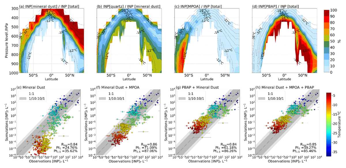
Figure 10
Top row: percentage contribution of each species to the total INP concentration (a–d), calculated using multi-year averaged zonal mean profiles of INP number concentration at modelled ambient temperatures. Panels show the contribution of: (a) quartz and feldspar, (b) the relative contribution of INP from quartz within the quartz and feldspar, (c) marine bioaerosols and (d) fungal spores and bacteria. The black contour dashed lines show the annual mean temperature of the model. Bottom row: Comparison of INP concentrations calculated at the temperature of the measurements against observations accounting for mineral dust (e), mineral dust and MPOA (f), mineral dust and PBAP (g) and all these combined (g). The dark grey dashed lines represent one order of magnitude difference between modelled and observed concentrations, and the light-grey dashed lines depict 1.5 orders of magnitude. The simulated values correspond to monthly mean concentrations, and the error bars correspond to the error of the observed monthly mean INP values. The colour bar shows the corresponding instrument temperature of the measurement in Celsius. Pt1 and Pt1.5 are the percentages of data points reproduced by the model within an order of magnitude and 1.5 orders of magnitude, respectively. Correlation coefficient is denoted with R, which is calculated with the logarithm of the values. Figure adapted from Chatziparaschos et al. (2025) under the Creative Commons 4.0 (CC 4.0) license.
In Chatziparaschos et al. (2025) TM4-ECPL was further developed to investigate the importance of marine primary organic aerosol (MPOA), and terrestrial primary biological aerosol particles (PBAP) for ice nucleation in MPCs based on the parametrisations of Wilson et al. (2015) and Tobo et al. (2013), respectively. INP originating from PBAP were estimated to be the primary source of INP at low altitudes between –10°C and –20°C (Figure 10d), while INP from marine bioaerosol dominate in the Southern Hemisphere (SH), particularly at low altitudes at subpolar and polar latitudes, having maximums at temperatures around –16°C (Figure 10d). When compared with available global observational INP data, the model demonstrates its highest predictive power across all temperature ranges when both dust and MPOA are included (Figure 10f). The inclusion of PBAP slightly decreases the model performance (Figure 10g) by overestimating INP concentrations. However, it should be noted that PBAP could be a key contributor to ice nucleation events (Figure 10d) at warmer temperatures despite the large uncertainties in its parameterisations (Chatziparaschos et al., 2025).
The INP schemes for quartz, K-feldspar (Harrison et al., 2019) and MPOA (Wilson et al., 2015) were then implemented in the EC-Earth3-AerChem model in combination with a secondary ice production parametrisation (Sect. 3.7.2, Georgakaki and Nenes, 2024), replacing the deposition-condensation-freezing temperature-based parametrisation by Meyers et al. (1992). Simulations demonstrate improved agreement with INP observations when using a parametrisation that accounts for the sensitivity of heterogeneous ice nucleation to mineral dust (K-feldspar and quartz) and marine organic aerosols, as opposed to the traditional temperature-dependent approach. To summarise: Our findings support the inclusion of aerosol aware INP parametrisations into ESMs, in particular for dust (K-feldspar and quartz), but also potentially for PBAPs and MPOA (Chatziparaschos et al., 2023, 2025), however their sources remains highly uncertain. The applicability of this recommendation naturally depends on the description of dust and primary particle sources within a given ESM.
3.7.2 Secondary ice production processes
Observations of significant numbers of ICNCs that significantly surpass the concentration of INPs in warm MPCs (at around –25°C and above) most likely indicate the presence of SIP. It is therefore recommended that key SIP processes are included in regional and global climate model simulations. However, how much the addition or refinement of a single process can improve model results depends on the model’s structure and other included processes. For example, the studies by Proske et al. (2022, 2023) identified SIP as one potential candidate for simplification (among others), at least within the context of the current representation of ice formation processes in ECHAM-HAM (See Sect. 2.1.3 and Table S7). That is because other processes dwarf SIP’s influence on key global cloud variables in this specific model. Ongoing work utilising all three FORCeS models (Ickes et al., 2025) highlights the intricate interconnections between all relevant cloud microphysical processes: the impact of modifying a specific process within one model may vary significantly from its effect in another model with a different microphysics scheme. Further research and exploration of this topic and the level of detailed required in various applications is therefore warranted.
Initial comparisons within FORCeS between observed ice-phase cloud properties during the NASCENT campaign (Sect. 2.2.1), obtained using a holographic imager mounted on the tethered balloon system (Pasquier et al., 2022a), and simulations from the Weather Research and Forecasting (WRF, Sect. S2.3) model (Skamarock et al., 2021) revealed that the model’s representation of these properties is inadequate without fine-tuning the cloud microphysics scheme (Schäfer et al., 2024). Indeed, measurements taken in Ny-Ålesund highlighted the importance of SIP in the form of drizzle shattering in Arctic MPCs (Pasquier et al., 2022a), and also pointed out the complexity of the shape of the ice crystals affecting their radiative properties (Pasquier et al., 2023). Focusing on a single cloud event, Schäfer et al. (2024) performed WRF simulations with two different microphysics schemes (Milbrandt and Yau, 2005; Morrison, Thompson and Tatarskii, 2009), constrained by observed CCN and INP concentrations. Their simulations underscored the necessity of accurately representing both primary and secondary ice formation processes in the model. The best alignment with observed hydrometeor profiles and precipitation was achieved after enhancing the efficiency of the Hallett-Mossop (HM; rime-splintering) process and incorporating descriptions of collisional fracturing and breakup (BR) as well as droplet freezing and shattering (DS). These modifications were implemented in the Morrison microphysics scheme, following the methodologies of Sotiropoulou et al. (2021) and Georgakaki et al. (2022), respectively.
Similar results were obtained by Han, Hoose and Dürlich’s (2024) simulations for convective clouds with the ICON model (Sect S1.2) with parameterisations for BR and DS included. Recognising the critical role of SIP in polar MPCs and the need for their accurate representation in large-scale models led to the development of the Random Forest SIP parametrisation (Georgakaki and Nenes, 2024). RaFSIP is a data-driven parametrisation created using machine learning techniques, leveraging comprehensive mesoscale WRF simulations with advanced SIP descriptions. This work is presented in detail in Georgakaki and Nenes (2024) and thus a short overview is given here.
The development of RaFSIP was based on a training dataset derived from two years of regional climate simulations using the WRF model, focusing on polar stratiform clouds across the pan-Arctic region from 2016 to 2017. Two nested domains were employed (Figure 11), and cloud microphysics were parameterised using an updated version of the Morrison, Thompson and Tatarskii, (2009) scheme including the three most significant SIP processes: HM, BR and DS (Georgakaki, Sotiropoulou and Nenes, 2024). Two variations of the RaFSIP scheme were developed: RaFSIPv1, which indirectly expresses the effect of SIP through the so-called Ice Enhancement Factor, and RaFSIPv2, which directly predicts SIP rates (see Georgakaki and Nenes, (2024), for details). These both consider SIP in temperatures as low as –25°C, as supported by the recent observational findings (Korolev et al., 2022; Pasquier et al., 2022a; Wieder et al., 2022). As demonstrated in Figure 11, the absolute differences between the ICNCs predicted by the detailed SIP microphysics simulation of WRF (referred to as ALLSIP) and those predicted by the simulation that ran with RaFSIPv2 (referred to as RaFSIP) demonstrated that RaFSIP effectively replicates the mean horizontal distribution of ICNCs, with mean biases below 30 # L–1. These biases in modelled cloud-phase partitioning do not appear to translate into significant radiative biases. The largest radiative biases were observed during the summer (Figure 11d), compared to the slower build-up (Figure 11b) and Arctic Haze periods (Figure 11c), likely due to slight differences in the glaciation fraction of the simulated clouds, which allowed more shortwave radiation to reach the surface.
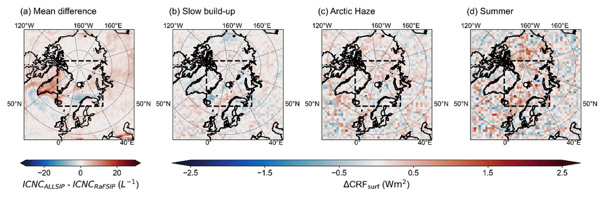
Figure 11
The first panel (a) shows the difference between mean ice crystal number concentrations predicted by the detailed microphysics simulation of WRF (ALLSIP) minus the simulation that ran with RaFSIPv2. The mean is derived from the entire year of simulations (September 2019–August 2020), focusing on the cases where: ICNC > 10–5 L–1 and temperature was between –25°C and 0°C (where ice multiplication was enabled in the WRF model). Panels (b) to (d) show the radiative biases in the predicted cloud radiative forcing at the surface calculated for the three periods: slow build-up (October–January), Arctic haze (February–May), and summer (June–September). Figure is adapted from Georgakaki and Nenes (2024) under the Creative Commons 4.0 (CC 4.0) license.
The design of the RaFSIP scheme allows for straightforward implementation in the dynamical core of any ESM that lacks detailed microphysics, as long as the relevant input features (i.e. temperature and RH with respect to ice) are properly integrated within the stratiform cloud microphysics routine. Our recommendation is therefore that the RaFSIP v2 scheme, as presented by Georgakaki and Nenes, (2024), should be used for a comprehensive emulation of SIP processes in ESMs. The RaFSIP approach outlines a way towards model simplification that can maintain the “essence” of complex physics in model versions that require limited complexity. Its design strikes a balance between detailed process representation and computational efficiency, making it a valuable tool for improving the accuracy of SIP in ESMs without the need for highly complex microphysics schemes.
Within FORCeS, RaFSIP has now been successfully incorporated into the microphysics modules of the three participating ESMs: EC-Earth3-AerChem, NorESM2 and ECHAM-HAM (see Table S1 in Sect. S7). Preliminary results from the model intercomparison study (utilising RaFSIPv2), however, show that the addition of a unified SIP parameterisation leads to varied model responses in terms of the simulated supercooled liquid fraction (Ickes et al., 2025). This highlights the complexity of microphysical process interactions as mentioned at the beginning of this section, and suggests that robust conclusions about real-world process importance cannot be drawn from individual models alone.
3.8 Recommendations for aerosol processing and scavenging by clouds
3.8.1 Aerosol number and mass scavenging by clouds and precipitation
Nucleation scavenging is the main loss mechanism affecting sub-micron aerosol particle number size distributions (Isokääntä et al., 2022; Tunved et al., 2013; Wang, Zhang and Moran, 2010; Wang, Xia and Zhang, 2021). This highlights the importance of getting CCN activation right in atmospheric models (see also Sect. 1.5 and 3.5). A systematic investigation of the implications of activation descriptions for wet scavenging and predicted aerosol size distributions in ESMs is therefore recommended (see also Sect 3.5). Studies using direct and simultaneous observations of total PM, cloud water and interstitial aerosol population suggest a less efficient uptake of BC to cloud water as compared with the more soluble components – probably due to effects of external mixing and the distribution of the BC material in the aerosol size distribution (e.g. Ruuskanen et al., 2021). Trajectory-based studies indicate that during cold seasons (T < 10°C) SO4, OA and BC are scavenged by precipitation equally efficiently in air masses arriving at Hyytiälä, Finland (Isokääntä et al., 2022; Talvinen et al., 2025), indicating internal mixing of these aged aerosol components. During the warm season (T > 10°C) SO4 is scavenged less efficiently than OA and BC indicating that SO4 might be distributed to smaller sizes than OA and BC (Isokääntä et al., 2022).
Similar relationships between precipitation and BC concentration as as well as overall number size distribution were also reported by Tunved et al. (2021) for Ny Ålesund in the Arctic. Heslin-Rees et al. (2024) followed on the work and showed that about 25% of the long-term trends of absorbing aerosol in the Arctic is explained by changing precipitation patterns. Together with the recent evaluation of a new wet scavenging scheme within ECHAM-SALSA (Holopainen et al., 2020) and the ongoing ESM intercomparison by Cremer et al. (2024) with regards to transport of BC to the Arctic, these results highlight the importance of an accurate description of the level of external mixing of soluble and insoluble compounds in modeled emissions and size-dependent composition of the aerosol population for getting the wet removal mechanisms right. Further studies on the size-dependent aerosol composition distribution and mixing state are therefore warranted to allow for the accurate description of aerosol-cloud interactions and wet removal.
A modelling closure between boundary layer dynamics, aerosol, and cloud properties can be achieved in well characterised cases such as those specified for the FORCeS 2020 campaign at the SMEAR IV site in Puijo, Finland (Calderón et al., 2022, see also Sect. 2.2.2). Observation-based sounding profiles were fundamental to achieve closure between large eddy simulations and observations of the cloud structure and the vertical wind velocity probability distribution. Likewise, the initialisation of aerosol properties using observation-based aerosol number concentrations and aerosol composition had a relevant role for obtaining closure of the activation efficiency curves. Moreover, as shown in Figure 12, the cloud droplet size distribution was also reproduced after accounting for the larger, supermicron aerosol particles, which produce drizzle most efficiently. As the effect of cloud processing on aerosol properties is difficult to observationally constrain, the findings support the further employment of models like UCLALES-SALSA (Sect S3.1) for the development of wet scavenging schemes accounting for different chemical compounds in global models. Simultaneous observations of atmospheric thermodynamic profiles (or updrafts) together with high-resolution measurements of aerosol number size distribution and chemical composition are important for obtaining closure for CCN activation and predicting cloud hydrometeor populations in liquid-phase clouds. Where possible, we therefore recommend the use of LES-type models for developing parametrisations for larger-scale models also, when it comes to wet scavenging. Given the importance of coarse mode aerosols for cloud microphysics and e.g., autoconversion (see also Sect. 3.6), LES-based closure studies could also help provide constraints on coarse-mode aerosol emissions and concentrations.
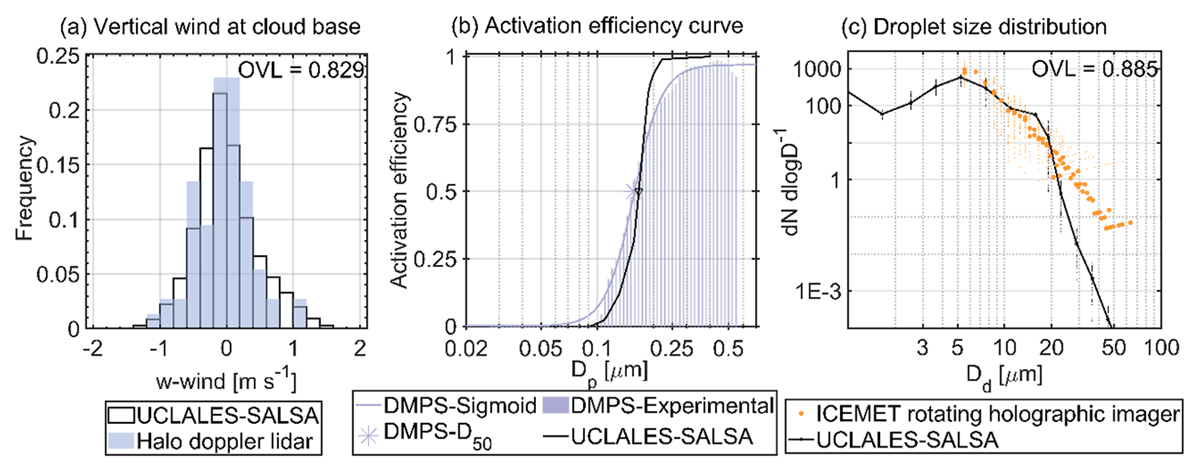
Figure 12
Modelled and observed cloud properties during the 5th hour of the cloud event of 24 September 2020 during the Puijo 2020 campaign. In (a), vertical wind at cloud base compared to Halo Doppler lidar observations is shown. Activation efficiency curve retrieved from Differential Mobility Particle Sizer observations with the twin-inlet system compared to modelled equivalent of total and interstitial aerosol particles is presented in (b). Droplet size distribution compared to observations with the ICEMET rotating holographic imaging system is shown in (c). Values of the overlapping index (OVL) have been added to indicate the degree of agreement between distributions. If two distributions are equivalent the OVL index tends to the unity.
3.8.2 Chemical processing and secondary aerosol generation within clouds
Aqueous formation of sulfate is visible in sub-micron aerosol in the boreal forest environment (Figure 13a), thus at least it is qualitatively in line with the mechanisms applied at present within the ESMs. The sulfate mass concentrations observed in Hyytiälä, Finland by Isokääntä et al. (2022) increased 44–61% due to in-cloud sulfate formation, and the increase was largest during the cold season and with more polluted air masses (Figure 13a and Isokääntä et al., 2022). The same conclusion (Figure 13b–c) was also obtained for two ESMs also utilised within FORCeS: UKESM1 and ECHAM6.3-HAM2.3-MOZ1.0 with the sectional aerosol module SALSA2.0 (Talvinen et al., 2025). In addition to increased sulfate mass, the mass fraction also increased (Figure 13d–f) implying changes in particle composition. The formed aerosol mass ended up between 200 and 600 nm in the aerosol size distribution, as expected from observations of cloud-processed sub-micron aerosol size distributions (Isokääntä et al., 2022). Aqueous-phase formation of sulfate has been implemented in ESMs since the 1990s. Based on previous work (e.g. Roelofs et al., 2006) and the work conducted within FORCeS, we recommend that the sulfate formed in the aqueous-phase should be distributed over the Aitken, accumulation and coarse modes. No signs of significant aqueous SOA formation, on the other hand, were observed in this boreal environment a) during the warmer season (T > 10°C) over areas with monoterpenes (MTs) dominating the biogenic volatile organic compound (VOC) emissions and total VOC; or b) during the colder season (T < 10°C) when anthropogenic emissions dominate over biogenic emissions (Isokääntä et al., 2022). Similar observations have also been made by Graham et al. (2020) for Swedish boreal forest environments. Based on studies within the boreal zone and the Arctic, no traces of significant aqueous SOA production have been observed and can therefore probably be neglected within these environments in ESMs. It is important to note, however, that aqueous-phase SOA is routinely observed and a well-established phenomenon in isoprene-dominated environments (e.g. Ervens, Turpin and Weber, 2011; Marais et al., 2016; Surratt et al., 2010).
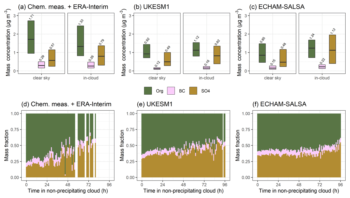
Figure 13
Top row: Median (black horizontal lines and numerical values) particle mass concentrations with 25th–75th percentiles (boxes) for OA (noted here, and in Isokääntä et al., 2022 as Org), eBC, and SO4 for the cold and polluted airmass sector at SMEAR II station, Hyytiälä, Finland. The experienced conditions by the air mass are denoted as clear sky and in-cloud (non-precipitating), and the data is temporally harmonised across observations and GCMs. Bottom row: The mass fractions of OA, SO4, and BC (derived from median concentrations at each 1-hour bin) for the more polluted air masses as a function of time spent in in non-precipitating cloud. Figure created from the data used in Isokääntä et al. (2022) and Talvinen et al. (2025).
3.8.3 Aerosol precursor scavenging by convective clouds
Understanding the details of trace gas transport through convective clouds is important for better predictions of upper tropospheric (UT) NPF as source of particle number at higher altitudes (see e.g. Williamson et al., 2019). In addition to the removal of particulate mass by clouds and precipitation, we have also investigated the processes that affect gas transport and removal within deep convective clouds (Bardakov et al., 2020, 2021, 2022, 2024; Wang et al., 2022).
Using the LES model MIMICA (Sect. S3.2), Bardakov et al. (2021) produced individual parcel trajectories within simulated deep convective clouds. A box model was then coupled to these trajectories to calculate e.g. gas condensation on hydrometeors, gas-phase chemical reactions, gas scavenging by hydrometeors and turbulent dilution. Trace gas transport followed approximately one out of three scenarios, determined by a combination of the equilibrium vapour pressure (containing information about water-solubility and pure component saturation vapour pressure) and the enthalpy of vapourisation for the ranges of molecular properties for isoprene system considered by Bardakov et al. (2021). At one extreme, the trace gas will eventually be completely removed by uptake to hydrometeors and precipitation. At the other extreme, there is almost no vapour condensation on hydrometeors and most of the gas is transported to the top of the cloud. Any physically-based description of scavenging by clouds should therefore couple effective volatility and chemical reactivity to the cloud liquid and ice water content in a dynamically evolving atmosphere.
Nucleation of organic species is one of the most important mechanisms contributing to the aerosol concentrations in the UT. Isoprene nucleation has been in focus with recent studies (Bardakov et al., 2024; Curtius et al., 2024; Shen et al., 2024), especially looking at the night-day transition. Before sunrise, a convective event can transport around 20% of the highly volatile isoprene emitted to the upper troposphere, as shown in Figure 14. Figure 14 displays the isoprene gas system surviving to the convective updraft, using the CloudChem box model (Sect. S3.3), with isoprene in blue (IVOC). After sunrise, isoprene is then oxidised to form large amounts of ultra-low volatility species, which can reach concentrations of about 107 molecules cm–3. Finally, these species directly nucleate at high rates and lead to typically observed nanoparticle concentrations of 103–105 particles cm–3 over the tropics (Andreae et al., 2018).
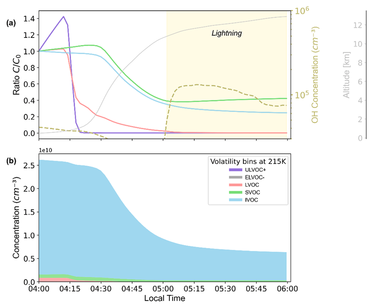
Figure 14
Transport of the isoprene gas-phase system during night-time convection over the Amazon. In (a) the fraction of the initial gas-phase concentration within volatility bins that survives night-time transport (chemistry and microphysics processes) is presented, and the altitude is shown with thin grey line and the OH concentration by the dashed olive yellow line. In (b) the contribution of different volatility bins to the total gas-phase concentration during transport is shown. Organic compounds are categorised according to their volatility with C* obtained for T = 215K: ULVOC+, extended ultra-low volatility organic compound, with the equilibrium saturation concentration C*(T) ≤ 3 × 10⁻⁷ μg m–3 (7 compounds) in purple; ELVOC-, reduced extremely low-volatility organic compound, with 3 × 10⁻⁷ < C*(T) ≤ 3 × 10⁻⁵ μg m–3 (1 compound = C4H5O3) in grey; LVOC, low-volatility organic compound, with 3 × 10⁻⁵ < C*(T) ≤ 0.3 μg m–3 (8 compounds) in red; SVOC, semi-volatile organic compound, with 0.3 < C*(T) ≤ 300 μg m–3 (1 compound = MVK/MACR = C4H6O) in green and the IVOC, intermediate volatile organic compound, with 300 < C* (T) ≤ 3 × 10⁶ μg m–3 (1 compound = Isoprene = C5H8) in blue.
The results from Bardakov et al. (2021) on the isoprene system also show that gas uptake to anvil ice is an important parameter for regulating the intensity of the isoprene oxidation and associated low volatility organic vapour concentrations in the outflow. This result is corroborated also by the study by Wang et al. (2022), which studied a completely different system, namely synergistic NPF of ammonia, nitric acid and sulfuric acids at high altitudes. This study suggests that transport of the trace gases through convective clouds, particularly ammonia, plays a large role in NPF in the upper troposphere in Asian monsoon. The trace gas scavenging onto ice is highly uncertain, and hence further studies on vapour uptake on and retention from ice hydrometeors are warranted.
The work towards parameterising the findings from the LES and box model frameworks discussed above for potential use in larger scale models is ongoing, in relation to, e.g., the descriptions of Jeuken et al. (2001) and Roelofs and Lelieveld (1995) that are currently used within EC-Earth. If NPF in the UT was to be explored within ESMs, the description of the transport and chemical transformation of the precursor VOCs in the convective systems needs to be explored and parameterised in a way that is physically consistent and in line with present observations (Bardakov et al., 2020, 2021, 2022, 2024; Curtius et al., 2024).
4 Summary, Conclusions and Outlook
Uncertainties in anthropogenic aerosol radiative forcing estimates are still a bottleneck for confidence in future climate projections (e.g. Im et al., 2021; Samset et al., 2018). One way to address this issue is to improve current descriptions of aerosol and cloud processes in Earth System Models (ESMs). Other key developments include increased model resolution, enhanced observational constraints and using simplified models and statistical emulation to obtain comprehensive yet computationally efficient parametrisations (see also Shaw and Stevens, 2025). In the framework of the FORCeS project, we reviewed current representations of aerosol and cloud processes (Figure 1) in a number of ESMs and scrutinised them against state-of-the-art knowledge. We then conducted new research to enhance our process understanding and to push the development of the model parametrisations. As a result, we arrived at a number of recommendations for ESMs regarding key chemical and microphysical processes. In the following, we summarise our recommendations, which are currently in various implementation phases within the ESMs covered in this article (see Sect. S7).
Organic aerosol (OA) is chemically complex and thus challenging to describe in models, yet important for climate feedbacks involving natural aerosol, for example, but also for capturing the sources and properties of human-driven emissions—including partly absorbing brown carbon (BrC), whose emissions remain particularly uncertain. Its representation is always a balance between an accurate enough description of the OA evolution and properties and limiting the number of additional tracers to include in the model. Our recommendation for ESMs is to consider implementing ORACLE-lite (Tsimpidi et al., 2025), especially if their current parametrisations do not consider the large variation in volatility of organic species. In addition, the approach developed for EC-Earth-AerChem by Bergman et al. (2022) focusing on two lumped species, namely semi-volatile and extremely low-volatile organic species might be of interest to models that seek an even simpler, yet thermodynamically-based representation of OA.
Particulate nitrate is expected to become more important in the future as reductions in anthropogenic SO2 emissions will increase the fraction of ammonium-containing species, such as ammonium nitrate. We therefore recommend adding nitrate to any ESM, but most importantly when simulating interactions between air quality and climate. The computationally efficient atmospheric aerosol thermodynamics module, ISORROPIA-lite (Kakavas, Pandis and Nenes, 2022; Milousis et al., 2024), developed within FORCeS, is well-suited for this purpose. As inorganic partitioning is often not included in ESMs, we recommend incorporating a thermodynamic model, such as ISORROPIA-lite, which offers reduced computational cost and good performance compared to the standard ISORROPIA-II. In applications in which accurate prediction of the distribution of nitrate between the fine and coarse modes is critical, we recommend reviewing relevant studies and considering the implementation of a dust mineralogy climatology.
For black carbon (BC), models should align with recent experimental findings. Liu et al. (2020) reviewed available literature on BC absorption properties and determined an average MAC of 8 ± 0.7 m2 g–¹ at 500 nm from ten different measurements. Regarding BrC, three different BrC species are ideally considered: two primary strongly absorbing species and one photobleached very weakly absorbing species, denoted as pbBrC. Based on current knowledge, the BrC from oxidation of aromatic VOCs could be neglected as a first approximation. The first primary BrC tracer (about 10% of the total BrC emission) to be considered is inert and insoluble and does not lose its absorbing properties. The second primary BrC tracer is soluble and loses its absorbing properties by photobleaching and is transformed to pbBrC. For this reaction, a rate constant k = 3.4 × 10⁻⁵ s–1 or a rate depending on OH radical concentration should be used. All BrC species to be considered are in the accumulation mode and are subject to atmospheric deposition. For improving the representation of the single scattering albedo of dust, we recommend updating optical constants using recent lab constraints (Di Biagio et al., 2019; Li et al., 2024a; Obiso et al., 2024) and calibrating absorption to observed iron oxide fractions. Models should incorporate region-specific soil mineral data, leveraging high-resolution datasets such as NASA’s EMIT mission. For computational efficiency, options include representing key iron oxides as separate tracers while grouping similar minerals (e.g. clays) or employing precomputed lookup tables to dynamically adjust optical properties. These approaches balance improved realism with manageable computational cost.
The representation of ultrafine aerosols and new particle formation (NPF) within ESMs varies; it can rely on semi-empirical parametrisations of field observations or laboratory observations of NPF involving known chemical systems or some combination thereof. The work conducted within FORCeS showed that Eq. (1) provides good results and can therefore be recommended if a field-based semi-empirical approach is desired. If a laboratory-based approach is desired, many of the experimental studies reviewed by Kirkby et al. (2023) have been cast into simplified parametrisations (Dunne et al., 2016; Gordon et al., 2016; Lehtipalo et al., 2018; Zhao et al., 2024), that can be utilised within larger-scale models such as ESMs. It is also important to ensure that Aitken mode dynamics are properly represented within ESMs, as smaller aerosols can act as cloud condensation nuclei (CCN), especially in cleaner environments. In the upper troposphere, these processes can be captured with NPF parametrisations derived for boundary layer conditions, but an accurate simulation requires proper representation of trace gas transport, chemistry, and also particle downward transport.
Accurate calculation of the number of activated droplets (Nact) is crucial for constraining the ACI forcing estimates, and thus the cloud droplet activation schemes in both GCMs (general circulation models) and ESMs should be carefully selected. Recent work by Ghosh et al. (2025) has shown that the complex iterative based droplet activation parametrisation of Morales Betancourt and Nenes (2014) and a modified version of Abdul-Razzak and Ghan (2000) scheme provide relatively good agreement with adiabatic cloud parcel models, and are therefore recommended for treating droplet activation in the FORCeS ESMs. Recent results highlight the importance of accurately characterising the aerosol lifecycle in models to ensure a realistic representation of the size distribution, which is crucial for droplet activation parameterisations. While models account for all aerosol modes, under certain conditions—such as clean environments—both Aitken and coarse mode particles can significantly contribute to CCN populations, and their influence may be underestimated if the input size distribution is not sufficiently resolved.
For liquid cloud microphysics, we obtained a number of insights that might be helpful in the development of cloud schemes in ESMs, but also in using and interpreting observations for model evaluation. The work conducted within FORCeS (Prank et al., 2022, 2025) supports earlier findings that giant CCN, and also coarse mode particles, are important to consider in autoconversion parametrisations for capturing the formation of drizzle correctly. For fog specifically, we recommend avoiding autoconversion parametrisations, especially if the fog droplet formation is simulated realistically based on physically valid parametrisations that account for radiative cooling at the top of fog, sedimentation and activation processes within the fog. FORCeS recommends that the impact of increased aerosol concentrations on droplet evaporation and mixing, and thus cloud droplet number concentration (CDNC), cloud liquid water path (LWP) and cloud fraction, should be examined against observations. The results from FORCeS suggest that great care should be taken when inferring LWP responses to aerosol from remote sensing data. However, by carefully selecting cloud cases with similar meteorological conditions and ensuring that cloud condensation nuclei concentrations are well-defined, changes in liquid water can also be reliably determined using satellite data.
The general understanding of primary ice formation processes has increased substantially in the past two decades (Lohmann and Diehl, 2006; Spracklen and Heald, 2014; Wang et al., 2014; Zhao and Liu, 2022). FORCeS findings support that ESMs should include aerosol aware INP (ice nucleating particle) parametrisations, for dust in particular, although large uncertainties remain in the representation of aerosol sources of INPs. A mismatch between observed ICNCs and INPs for mixed-phase clouds (MPCs) that are decoupled from the surface and lack seeding from upper-level clouds can be attributed to secondary ice production (SIP). To address this, we recommend that key SIP processes be incorporated into ESM simulations to better capture realistic ICNCs. A data-driven parameterisation trained on physically detailed WRF simulations is the RaFSIPv2 scheme, presented by Georgakaki and Nenes (2024), which parameterises the combined effects of the three dominant SIP mechanisms and is designed for straightforward implementation in large-scale models (e.g. with horizontal grid spacings >10 km). The use of RaFSIP can support ongoing efforts to improve the representation of MPCs in climate models and deepen our understanding of cloud-phase processes and their role in the climate system.
In addition to investigating the ways that aerosol perturbations influence atmospheric radiation and cloud microphysics, several studies within FORCeS targeted different aspects of aerosol and precursor gas scavenging and processing by clouds. FORCeS findings (Isokääntä et al., 2022; Talvinen et al., 2025) confirm the established importance of aqueous-phase sulfate formation within clouds and suggest that this source is well-captured by state-of-the-art approaches. Based on studies within the boreal zone and the Arctic (Graham et al., 2020; Isokääntä et al., 2022), however, no trace of significant aqueous secondary organic aerosol production was observed in these environments and can therefore probably be neglected for these regions in ESMs. Given the importance of upper tropospheric NPF, the description of the transport and scavenging of the relevant precursor gases through convective clouds is also highly relevant to represent. Any physically-based description of scavenging of gas-phase species by clouds should couple volatility, solubility and chemical reactivity to the cloud liquid and ice water content in a dynamically evolving atmosphere. Given the non-linearity of the associated phenomena, we recommend the enhanced use of high-resolution modelling such as LES for developing parametrisations for larger-scale models for wet scavenging. If such processes were to be explored within ESMs, the description of the transport and chemical transformation of the precursor VOCs in the convective systems needs to be explored and parametrised in a way that is physically consistent and in line with present observations.
Continued efforts are required in prioritising model development and evaluation. Although advocating for improving aerosol and cloud representation in ESMs, we realise that model development always faces a trade-off between partially contradicting goals: increasing the number and detail of representations to enhance representational accuracy; using the model to generate understanding; and increasing model performance (in terms of decreasing computing time or increasing the match with observations). In particular, representative accuracy leads to model complexity, which is sometimes problematic for various reasons: (1) complexity hinders the understanding of the model and the ability to generate understanding with it, (2) a more complex model includes more free parameters that allow for multiple equally plausible model realisations (equifinality), (3) including processes in large detail increases the risk of overinterpreting the processes that are included while overlooking those that are not, (4) increasing model detail may not be decreasing uncertainty and finally, (5) more complexity and authority from included processes conceal non-epistemic influences such as values and habits (Proske et al., 2023 and references therein). Thus, adding more detailed representation and complexity comes with a price. That being said, the results from the FORCeS project do demonstrate the importance of capturing the key drivers of ACI better in the next generation of ESMs: it is hard to imagine a substantial decrease in the uncertainties associated with ACI with ESMs that do not include physically reasonable and high-enough resolution descriptions of particle number size distributions, water vapour concentrations, emission sources (critically characterised and constrained by the chemical fingerprint present in the particles) and cloud microphysics (including hydrometeor size distributions and phase). The reduction in aerosol ERF uncertainty should also be targeted through addressing internal model inconsistencies and rigorous model evaluation procedures. Related to the former, structural errors in present ESMs may result in inconsistencies in key parameters for ACI, LWP and CDNC as examples. Such inconsistencies could be remedied with thoughtful application of high-resolution and LES modelling constrained by a combination of in-situ and remote-sensed observations. As needed, such developments can be facilitated with large ensemble simulations using e.g., statistical emulation. For model evaluation, multiple observation types should be used to avoid overfitting models to very limited sets of observations. Our results therefore demonstrate the importance of long-term, high-resolution empirical data (both in-situ and remote sensing) and the potential of using detailed process models to facilitate direct upscaling such observations for direct comparisons with ESMs (see e.g., Arola et al., 2022). Furthermore, we advocate prioritising process-based evaluation approaches that complement the traditional parameter-based evaluations (e.g., Blichner et al., 2024; Virtanen et al., 2025). Continued dialogue is needed between the research communities working with detailed microphysical and chemical processes relevant to the Earth system, and those developing and using global models. Likewise, our results have demonstrated the critical importance of open discussion on the limitations and potential of various data sets used for ESM evaluation, and have pinpointed areas where methodological developments are critical for pushing the research frontiers in this field of climate science.
Acknowledgements
We gratefully aknowlegde the key contributions from Trude Storelvmo, Ulrike Lohmann and David Neubauer during the FORCeS project. Sini Talvinen would like to extend personal thanks to Roman Bardakov from all the helpful discussions during the writing process of this work.
Competing Interests
The authors have no competing interests to declare.
Author Contributions
Ilona Riipinen and Annica M. L. Ekman proposed the study and designed the concept with contribution from Sini Talvinen.
Ilona Riipinen and Sini Talvinen wrote the original manuscript with support from Annica M. L. Ekman, Paraskevi Georgakaki, Carlos Pérez García-Pando, Ulrike Proske, Lubna Dada, Øyvind Seland, Daniel G. Partridge, Almuth Neuberger, Snehitha M. Kommula, Stefano Decesari and Twan van Noije.
The figures were created by Sini Talvinen together with Anouck Chassaing, Paraskevi Georgakaki, Xinyang Li, Tommi Bergman, Snehitha M. Kommula, Angelos Gkouvousis, Alexandra P. Tsimpidi, Marios Chatziparaschos, Almuth Neuberger, Vlassis A. Karydis, Silvia M. Calderón, Sami Romakkaniemi, Théodore Khadir and Paul Zieger.
All co-authors edited the manuscript and provided valuable feedback.