
Table 1
Summary of the categories and geographical boundaries of the ten different study regions. The three-letter codes listed will henceforth be the notation used.
| REGION | ABBREVIATION | CATEGORY | LONGITUDE-LATITUDE BOX | |
|---|---|---|---|---|
| 1 | Iceland | ISL | Volcanic | [–30, –10, 50, 70] |
| 2 | Hawaii | HWI | Volcanic | [–170, –150, 10, 30] |
| 3 | E. Europe | EEU | Anthropogenic | [15, 40, 35, 55] |
| 4 | E. US | EUS | Anthropogenic | [–80, –65, 30, 45] |
| 5 | E. China | CHN | Anthropogenic | [100, 123, 27, 42] |
| 6 | Australian | AUS | Stratocumulus | [95, 115, –35, –20] |
| 7 | Canarian | CAN | Stratocumulus | [–35, –25, 15, 30] |
| 8 | Namibian | NAM | Stratocumulus | [0, 15, –20, –10] |
| 9 | Peruvian | PER | Stratocumulus | [–90, –70, –25, –15] |
| 10 | Californian | CAL | Stratocumulus | [–130, –110, 20, 35] |
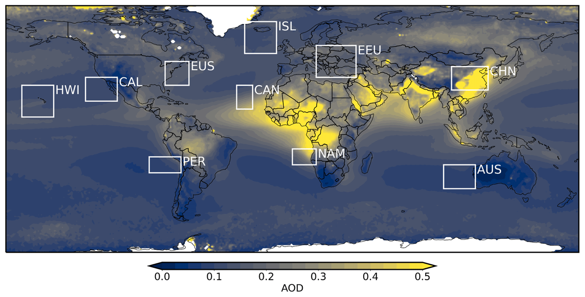
Figure 1
Regions included in the study. Mean AOD [unitless] between 2004–2020 is plotted in background for reference.
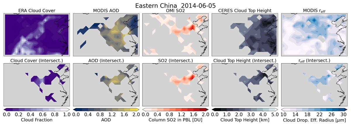
Figure 2
Data coverage for the different datasets included in the study. Top row shows each corresponding dataset for an example day in the CHN region. On each day, the model is only given data where all datapoints are available in all data sets (bottom row).
Table 2
Selected (in bold) and tested hyperparameters for the gradient boosting regression method.
| MODEL PARAMETER | VALUES |
|---|---|
| Learning rate | [0.0125, 0.025, 0.05, 0.1 ] |
| Number of boosting stages | [500, 750, 1000, 1250, 1500 ] |
| Max depth of individual estimators | [6, 9, 12, 15, 18] |
| Minimum samples to split internal node | [0.00001, 0.0001, 0.001, 0.01] |
| Minimum samples per leaf | [0.00001, 0.0001, 0.001, 0.01] |
Table 3
Selected (in bold) and tested hyperparameters for the neural network method.
| MODEL PARAMETER | VALUES |
|---|---|
| hidden layer sizes | [10, 10], [25, 25], [50, 50], [100, 100], [250, 250], [500, 500], [10, 10, 10], [25, 25, 25], [50, 50, 50], [100, 100, 100], [10, 10, 10, 10], [25, 25, 25, 25], [50, 50, 50, 50], [100, 100, 100, 100] |
| alpha | 1.0e-8, 1.0e-7, 1.0e-6. 1.0e-5, 1.0e-4, 1.0e-3 |
Table 4
Scores for gradient boosting regression model (R2, and NRMSE) for models with only meteorological input from ERA, with added air mass information (encompassing AMO and ztop), and with added aerosol information (encompassing AOD, SO2 and SO4).
| ERA ONLY | ERA + AEROSOL | ERA + AIR MASS | ERA + AIR MASS + AEROSOL | |||||
|---|---|---|---|---|---|---|---|---|
| REGION | R2 | NRMSE | R2 | NRMSE | R2 | NRMSE | R2 | NRMSE |
| ISL | 0.505 | 0.207 | 0.519 | 0.204 | 0.527 | 0.202 | 0.541 | 0.200 |
| HWI | 0.295 | 0.194 | 0.336 | 0.188 | 0.308 | 0.192 | 0.349 | 0.187 |
| EEU | 0.159 | 0.295 | 0.176 | 0.292 | 0.193 | 0.288 | 0.209 | 0.286 |
| EUS | 0.327 | 0.270 | 0.344 | 0.267 | 0.356 | 0.264 | 0.370 | 0.261 |
| CHN | 0.191 | 0.308 | 0.233 | 0.301 | 0.220 | 0.303 | 0.253 | 0.296 |
| AUS | 0.497 | 0.215 | 0.523 | 0.210 | 0.534 | 0.207 | 0.556 | 0.202 |
| CAN | 0.381 | 0.215 | 0.428 | 0.206 | 0.419 | 0.208 | 0.463 | 0.200 |
| NAM | 0.378 | 0.259 | 0.396 | 0.255 | 0.420 | 0.250 | 0.436 | 0.246 |
| PER | 0.583 | 0.252 | 0.617 | 0.241 | 0.636 | 0.235 | 0.659 | 0.228 |
| CAL | 0.422 | 0.289 | 0.442 | 0.284 | 0.475 | 0.276 | 0.492 | 0.271 |
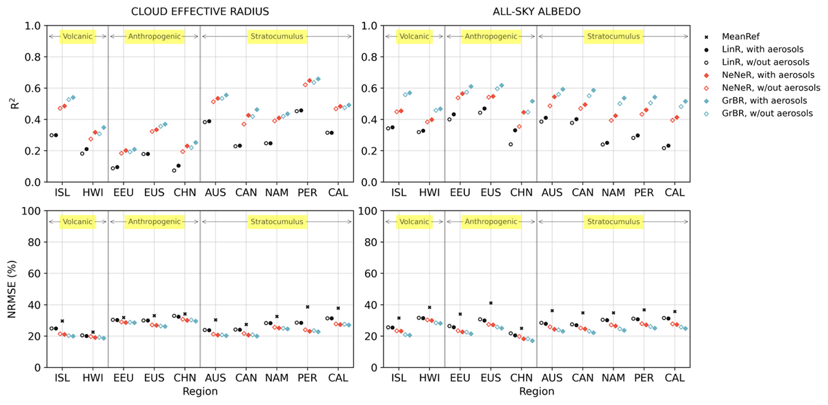
Figure 3
Model evaluation comparing R2 and normalised RMSE scores for NeNeR (red) and GrBR (blue) with a simple linear regression (black circles) and a mean reference model (black cross) for the two response variables reff (left) and all-sky albedo (right). Filled markers represent models with aerosols included and empty markers are models excluding aerosols. Regions are grouped according to their respective category.
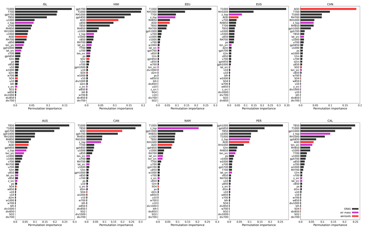
Figure 4
Permutation feature importance for prediction of reff in 10 regions. Meteorological input from ERA5 is marked black, whereas air mass variables (latsrc, lonsrc, zsrc, and ztop) are indicated in magenta, and aerosol variables (AOD, SO2 and SO4) are marked with red. Note the different ranges for the different regions.
Table 5
Mean values of AOD for the ten study regions, and direction of AOD impact on predicted reff (Negative (–) indicating cases where reff is smaller for higher aerosol burden, as expected from Twomey theory, and vice versa.). Feature importance rank of AOD, SO2 and SO4 respectively, out of 34.
| REGION | MEAN AOD | SIGN | RANK AOD | RANK SO2 | RANK SO4 |
|---|---|---|---|---|---|
| ISL | 0.140 | –/+ | 11 | 30 | 26 |
| HWI | 0.133 | – | 5 | 19 | 24 |
| EEU | 0.215 | + | 6 | 34 | 31 |
| EUS | 0.179 | –/+ | 4 | 33 | 27 |
| CHN | 0.636 | + | 1 | 22 | 26 |
| AUS | 0.094 | – | 8 | 33 | 23 |
| CAN | 0.213 | –/+ | 3 | 32 | 25 |
| NAM | 0.236 | –/+ | 8 | 33 | 23 |
| PER | 0.106 | – | 7 | 32 | 29 |
| CAL | 0.111 | –/+ | 7 | 33 | 31 |
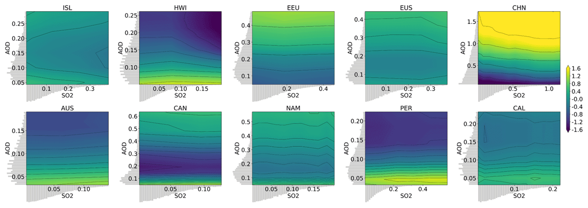
Figure 5
reff dependence on air mass source region (longitude and latitude anomalies) for all ten regions, outlined by white boxes. Grey shading indicates relative distribution of longitude and latitude origin values. The discontinuity at 0° longitude is due to the model being trained on longitudes from 0° to 360° rather than –180° to 180°.
Figure 6
reff (colour and contours) dependence on aerosols (AOD and SO2 anomalies) for all ten regions. Grey shading indicates relative distribution of AOD and SO2 values.