
1 Introduction
Aerosol-cloud interactions and their effects on Earth’s radiation balance remain one of the main uncertainties in future climate projection (Bellouin et al. 2020, Forster et al. 2021, Bender 2020). This is not only because future changes in aerosol loading are not known but also because the sensitivity in clouds to aerosol changes is uncertain. Investigation of aerosol-cloud interactions on large scale relies on more or less complex versions of correlation analysis, making it difficult to isolate and assess causality of aerosol effects, and to distinguish any potential signals from variation due to meteorological factors, that often co-vary with aerosols, and aerosol influence on cloud (Mauger and Norris 2007, Engström and Ekman 2010, Koren et al. 2010, Zhang et al. 2022). Attempts to account for varying meteorology are continuously made, e.g. by segregating analysis based on meteorological regime or time interval (Gryspeerdt and Stier 2012, Chen et al. 2014, Oreopoulos et al. 2017, Malavelle et al. 2017, Oreopoulos et al. 2019, Douglas and L’Ecuyer 2019, Chen et al. 2022) or like Gryspeerdt et al. (2014) rather investigating how the occurrence of and transition between different regimes varies with aerosol. Still, the challenge to separate meteorological variation from aerosol influence remains unsolved.
Methods from data science provide new ways of studying aerosol-cloud interaction, and here we apply machine learning techniques on large sets of reanalysis and remote sensing data to investigate the relative importance of meteorological and aerosol-related parameters in determining cloud microphysical properties over different geographical regions. Specifically, a gradient boosting regression (GrBR) model is trained to predict the cloud droplet effective radius (reff) supplied from the MODIS satellite-based record for each region. The GrBR is also compared with a neural network approach. As input parameters to the machine learning models, we use meteorological parameters such as temperature, humidity, geopotential height and wind on 1000 hPa, 850 hPa and 700 hPa from the ERA5 Reanalysis dataset together with deduced air mass origin (AMO) from the HYSPLIT trajectory model, and cloud top height (ztop) as well as aerosol optical depth (AOD) from MODIS, sulfur dioxide (SO2) concentration data from satellite-borne OMI, and near-surface sulfate mass concentration (SO4) from the MERRA-2 reanalysis.
The questions addressed in this study are the following:
Can a simple machine learning model predict a cloud microphysical parameter (reff) based on large scale meteorological variables alone, with any skill?
Will this model perform better when also given information about aerosol burden?
What is the relative importance of each parameter in predicting the model output?
We focus on the instantaneous effect of aerosols on cloud droplet formation and size, and thereby cloud reflectivity. All else equal – in particular, with constant liquid water path in the cloud – a higher aerosol loading is expected to give rise to clouds with more numerous and smaller droplets, with higher reflectivity (cloud brightening, Twomey 1974). A number of observational studies illustrate cloud brightening from aerosols, particularly discernible in so-called opportunistic experiments, such as volcanic eruptions or ship tracks, where well-defined aerosol perturbations occur in otherwise undisturbed environments, e.g. McCoy and Hartmann (2015), Toll et al. (2019), Diamond et al. (2020), Christensen et al. (2022), although the generalisability of such experiments to climatological forcing estimates has been questioned (Toll et al. 2017, Glassmeier et al. 2021). The adjustment of clouds to smaller droplets, through the competing effects of precipitation suppression and enhanced entrainment, adds additional uncertainty, by altering the amount of water in the clouds, and thereby potentially violating the assumption of constant liquid water path. Although there is evidence that thickening and thinning closely compensate under some conditions (Toll et al. 2017), the current study cannot assume a constant cloud thickness, and unaccounted for variations in liquid water path may interfere with the sought aerosol-signal.
As a measure of aerosol abundance we here use AOD, the total amount of aerosol extinction in the vertical column, that is expected to contribute negatively in the constructed models, so that large AOD values lead to predictions of smaller values of reff. While AOD is for several reasons not an ideal proxy for concentration of cloud condensation nuclei (CCN) (Liu and Li 2014, Shinozuka et al. 2015, Stier 2016, Quaas et al. 2020), it here serves the purpose of indicating the level of particulate matter (due to pollution, or from natural sources) present in the given regions and times. By comparing the prediction skill of models with and without aerosol information included, we can test both whether the aerosol information improves the model, and if so what the sign of the impact is. As a complement to AOD, that is an integral optical measure of aerosol loading, we also include SO2 concentration as additional input. SO2, that can oxidize to sulfate and co-varies with sulfate aerosol in time and space, can provide an independent indication of CCN-relevant aerosol signature (Aas et al. 2019, McCoy et al. 2018). In addition, we include reanalysis estimates of SO4, which has previously been shown to co-vary with cloud droplet number concentration on larger spatial and temporal scale (McCoy et al 2017, 2018).
With similar focus on processes determining cloud property variations, machine learning methods have been applied for instance by Fuchs et al. (2018) who use gradient boosting regression trees to quantify the importance of different cloud controlling factors in determining cloud fraction and droplet size over the Southeast Atlantic. Andersen et al. (2017) use an artificial neural network to predict cloud occurrence from satellite data and reanalysis fields, on near-global monthly mean scale, and in Andersen et al. (2023) ridge regression was applied to monthly, regional mean data over the same 60°S to 60°N domain, to quantify sensitivity of cloud radiative effects to a number of cloud controlling factors, including aerosol proxies. Focusing on the Southeast Pacific, Jesson et al. (2021) suggest that links between AOD, cloud properties and environmental factors can be explored using non-linear causal models.
Here, we don’t address causality but simply investigate the plausibility of predicting cloud properties from data describing the environmental conditions, and the importance of various types of input parameters in that prediction. As opposed to Fuchs et al. (2018) who focus on the sub-regional variability in a specific subtropical area, we perform our analysis on a set of regions that represent varying meteorological conditions and aerosol signatures (cf. Bender et al. 2019), and as opposed to (Andersen et al. 2017, 2023) we study daily resolved data, and make sure that satellite and reanalysis data are synchronised within hours in time.
We use a gradient boosting regression model (GrBR, described in Section 2.1) with input data from reanalysis and satellite records (described in Section 2.5), and compare it to a reference linear regression model (discussed in Section 2.3) and a neural network regression (NeNeR, described in Section 2.2). Section 2.6 discusses the optimisation of model hyper-parameters for the GrBR model as well as the NeNeR. In Section 3.1 we evaluate the GrBR model performance and in Section 3.2 we investigate the influence of including aerosol information as model input.
2 Methods and data
2.1 Gradient boosting regression
A GrBR model is trained to predict cloud droplet effective radius. Gradient boosting, as described e.g. by Friedman (2001), Hastie et al (2017), Géron (2019) works by combining a number of decision trees into one model. Following the initial model, each additional tree is trained to minimise the residual in the previous model, adding layers iteratively. Each new layer is fit to the negative gradient of the specified loss function, in this case the mean square error between model output and observations. The gradient boosting thereby combines weaker predictors into a single, more powerful model. Essentially, the model begins by simply considering the model output to be the average of the training set. The model then builds a slightly larger decision tree, combining it with the previous tree, using a scaling factor. Additional trees are added until the specified maximum number of layers is reached, or until the model score no longer improves significantly (Géron 2019).
The GrBR model is chosen here because of its decision tree structure providing predictive power and simple implementation, without requiring assumptions on input data distribution (cf. Zipfel et al. 2022). The decision tree structure also provides a way to determine how much each parameter contributes to the model’s final output. Because of the structure of the model, with decision trees that are based on parameter values, the contribution of each parameter to the model output can be extracted. Here, we illustrate this using permutation feature importance, which is a measure of the decrease in model score resulting from a random shuffling of a given parameter, and thereby can indicate the level of importance of each individual parameter for the outcome of the model.
To avoid overfitting, a clear distinction needs to be made between the data that the model is trained on, and the data used for testing. If this is not done, the model would simply repeat the labels of the samples that it has already seen during the learning process. Here, a randomly selected set of 20% of the data is set aside for testing, and given to the model only at the final evaluation stage. We note that random splitting of temporally structured data may underestimate error in extrapolative model building (Roberts et al. 2017), but for our interpolative purposes, there is less motivation for non-random splitting of the data, and we follow the examples of e.g. Fuchs et al. (2018), Chen et al. (2022) who randomly select training, test and validation data.
The GrBR models are set up in Python using Scikit (Pedregosa et al. 2011).
2.2 Neural network regression
The GrBR model performance is also compared to that of a NeNeR. As described in eg. Rumelhart et al. (1986); Géron (2019), a neural network consists of several layers; an input layer, a certain number of hidden layers and an output layer. Each layer consists of several nodes (or perceptrons) and the input as well as the hidden layers have an additional bias node.
The nodes of the input layer (usually one per feature) multiply the input value with a weight value and forward this result to the first hidden layer. Those values are then used as the input values for the perceptrons in the following hidden layer. Using the weighted sum of the input values, a so called ‘activation function’ is applied to produce a new output value which is then forwarded to the perceptrons in the next hidden layer. This is continued until the last layer, the output layer, is reached. While fitting the model with the training data set, the weights and bias are calculated (fitted) by minimizing a certain loss function, here the squared error. When a neural network is used for a single output regression the output layer consists only of one perceptron which evaluates the final predicted value. The architecture of a neural network can be expressed by a linear equation system, but by using an appropriate non-linear activation function the method can represent theoretically any continuous function and is therefore suitable to represent non-linear problems. For the neural network model, a standardization of the input data is required (Géron 2019), and here the data are normalised to a mean of zero and standard deviation of one.
The NeNeR models are set up in Python using Scikit (Pedregosa et al. 2011).
2.3 Linear regression
A linear regression model is used as a reference, to which the machine learning model performance can be tested. The linear regression is based on standardized data, sampled into a training set (n = 100,000) and a test set.
A separate and more extensive linear regression analysis is performed on the data to explore how much the linear model can be reduced without loss of performance (similar to a feature selection). To account for co-linearity between the variables in the regression model, a step-wise backward elimination, starting from the full model, is performed, where predictors are removed iteratively until all predictors are statistically significant (p = 0.05). Next, any remaining predictors are removed if they exhibit co-linearity with other predictors, accepting only variables for which the variance inflation factor is less than 5. This reduced model is tested alongside the full model.
2.4 Study regions
Ten geographic regions are selected to be used in the models. These are divided into three different categories based on cloud or aerosol properties specific to the region; volcanic influence, anthropogenic influence and stratocumulus regions. The first includes two areas with active volcanoes, the second covers three areas under immediate influence of anthropogenic emissions and the third comprises five subtropical stratocumulus regions, modified from Klein and Hartmann (1993). Table 1 lists the different regions and categories as well as the latitudes and longitudes defining each region’s bounding box, also indicated in Figure 1. The choice of regions was guided by previous research (e.g. Bender et al. 2019). The regions are chosen so that their sizes are large enough to have sufficient data for the model to train on, but still small enough to be subject to similar meteorological conditions.
Table 1
Summary of the categories and geographical boundaries of the ten different study regions. The three-letter codes listed will henceforth be the notation used.
| REGION | ABBREVIATION | CATEGORY | LONGITUDE-LATITUDE BOX | |
|---|---|---|---|---|
| 1 | Iceland | ISL | Volcanic | [–30, –10, 50, 70] |
| 2 | Hawaii | HWI | Volcanic | [–170, –150, 10, 30] |
| 3 | E. Europe | EEU | Anthropogenic | [15, 40, 35, 55] |
| 4 | E. US | EUS | Anthropogenic | [–80, –65, 30, 45] |
| 5 | E. China | CHN | Anthropogenic | [100, 123, 27, 42] |
| 6 | Australian | AUS | Stratocumulus | [95, 115, –35, –20] |
| 7 | Canarian | CAN | Stratocumulus | [–35, –25, 15, 30] |
| 8 | Namibian | NAM | Stratocumulus | [0, 15, –20, –10] |
| 9 | Peruvian | PER | Stratocumulus | [–90, –70, –25, –15] |
| 10 | Californian | CAL | Stratocumulus | [–130, –110, 20, 35] |
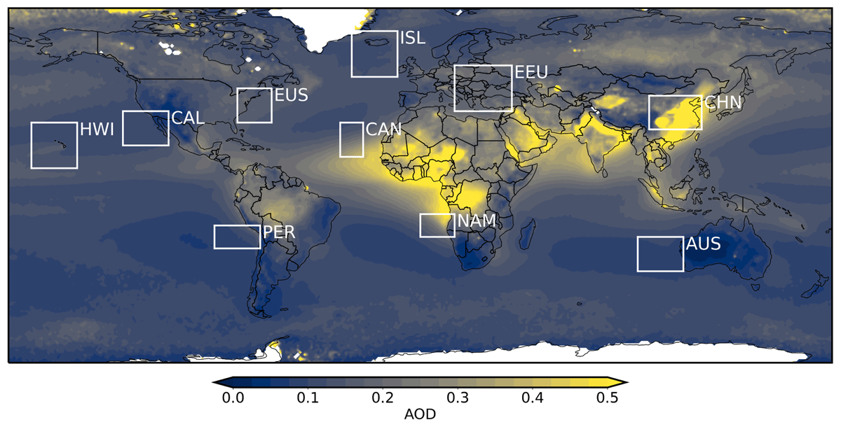
Figure 1
Regions included in the study. Mean AOD [unitless] between 2004–2020 is plotted in background for reference.
2.5 Data
Input data for the models come from ERA5 meteorology, MERRA-2 aerosol fields, MODIS and OMI satellite retrievals, and the HYSPLIT trajectory model, as described in the following. Output data (reff and albedo) come from MODIS/CERES.
For each of the model types (GrBR, NeNeR and linear regression), the analysis is carried out repeatedly for each region, with different combinations of input variables, to illustrate the relative importance of meteorological and aerosol information.
2.5.1 ERA5 meteorology
The meteorological parameters are obtained from the European Centre for Medium-Range Weather Forecasts (ECMWF) ERA5 reanalysis dataset (Hersbach et al. 2020) and include 700, 850 and 1000 hPa level temperature (T700, T850, T1000), relative humidity (RH700, RH850, RH1000), geopotential height (gph700, gph850, gph1000), zonal wind speed (u700, u850, u1000), meridional wind speed (v700, v850, v1000), vertical wind speed (w700, w850, w1000) and divergence (div700, div850, div1000). Noting that the 1000 hPa level is in several instances sub surface, in particular in the CHN region, we also include surface level information, namely 2-meter temperature (t2m), 2-meter dew point temperature (d2m), 10 meter horizontal wind speeds (u10, v10), estimated boundary layer height (blh), and surface pressure (ps). The meteorological parameters are selected at time steps corresponding to satellite overpass.
The pressure levels are chosen to describe the current synoptic, and local, weather situation while being low enough in the atmosphere for potential clouds to be liquid rather than ice phase. Our goal is to investigate how the cloud properties are determined by meteorology in a general sense, in contrast to aerosol. The input variables therefore don’t target specific processes or cloud controlling factors (as in e.g. Stevens and Brenguier (2009), Klein et al. (2017), Ceppi and Nowack (2021), Scott et al. (2020), Myers et al. (2021), Wall et al. (2022), McCoy et al. (2023), Blanco et al. (2023)), but are rather standard variables chosen to produce a general picture of the meteorological situation.
2.5.2 Satellite derived aerosol, cloud and radiation information
AOD and reff are retrieved from the MYD08 level 3 dataset from the Moderate resolution Imaging Spectroradiometer (MODIS) Collection 6 product (Levy et al. 2013, Platnick et al 2017). The AOD product combining the Dark Target and Deep Blue algorithm is used. MODIS observes a swath approximately 2330 km wide, but all data are aggregated to a horizontal resolution of 1° × 1°. The data used comes from MODIS carried on the Aqua satellite, which crosses the equator at the same local time every orbit, nominally at 1.30 pm, and makes between 14 and 15 orbits per day. However, the time it passes over a certain region of study varies each day by up to 2 hours. Thus, there is a slight discrepancy of the valid time of the meteorological reanalysis data and the satellite flyover time.
Important to note is that the MODIS instrument cannot retrieve aerosol data in a cloud-covered pixel. A consequence is that when studying the daily data of AOD, it often contains gaps where the satellite is unable to determine the aerosol content in the gridbox. This in turn means that the data used to feed the machine learning model is limited by the MODIS AOD coverage. This is illustrated in Figure 2.
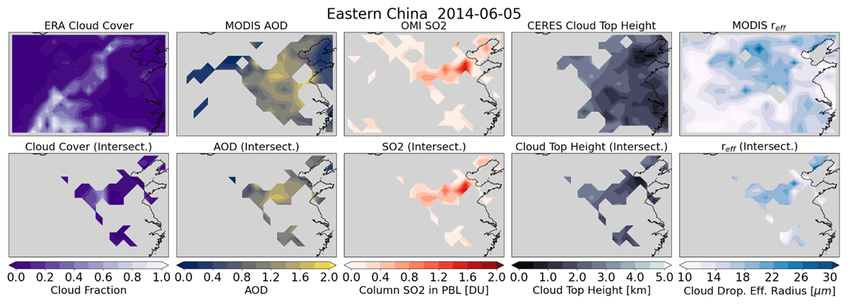
Figure 2
Data coverage for the different datasets included in the study. Top row shows each corresponding dataset for an example day in the CHN region. On each day, the model is only given data where all datapoints are available in all data sets (bottom row).
SO2 information is derived from the level 3 1-day Total Column Density of SO2 in the Planetary Boundary Layer (PBL) dataset measured by the Ozone Monitoring Instrument (OMI; Krotkov et al. 2016). OMI is a nadir-viewing instrument on board the NASA Aura satellite flying in the same sun-synchronous polar orbit as Aqua, with the equator-crossing time of 1.45 pm. The data are resolved with a resolution of 0.25° × 0.25°, but here interpolated onto a coarser 1° × 1° degree grid to match the MODIS dataset.
Because of limited spatial coverage of the OMI data, a 7-day rolling mean was calculated for SO2. Seven days was chosen as a compromise between short enough averaging time to maintain a signal of day-to-day variation, while not loosing too much data due to poor coverage.
In addition, however, the OMI SO2 data set contains a substantial amount of negative values, that are also filtered out, as they are considered unphysical. Spurious negative values in the OMI retrievals may appear in particular at the edges of clouds, due to corrections in measured radiance, and in high latitude regions due to high ozone concentration and/or large solar zenith angle (NASA n.d.). Further, the intrinsic noise in OMI produces noise in the SO2 measurements that exceeds most anthropogenic signals, with a standard deviation of 1.2–1.5 DU in tropical regions (OMI 2012). Therefore, the SO2 parameter can be expected to have a detectable impact on output mainly in regions with high levels of anthropogenic pollution, or in the rare events of strong volcanic outgassing or eruptions. This further limits the data used to feed the machine learning model, as seen in Figure 2.
For ztop (used as additional input to the model) and albedo (used as alternative output) parameters, we use estimates of those quantities from the Clouds and the Earth’s Radiant Energy System (CERES) Single Scanner Footprint (SSF) Edition 4.1, level 3 product (Wielicki et al. 1996, Loeb et al. 2016). The data are collected by the Aqua satellite and were accessed through the NASA Langley Research Center Atmospheric Science Data Center. A low (sfc–700hPa) cloud top height parameter is chosen so as to stay within the pressure range of the previously selected meteorological parameters, which filters the data primarily on liquid (warm) clouds. Top of atmosphere all-sky albedo is the ratio between shortwave (0.2–5μm) reflected and incoming solar flux at the top of the atmosphere for all-sky conditions.
2.5.3 MERRA-2 sulfate estimates
Additional aerosol information is taken from the MERRA-2 reanalysis (Randles et al. 2017), that includes vertically resolved estimates of mass concentration of five aerosol types, including sulfate. This follows McCoy et al (2018), who illustrated the predictive power of reanalysis SO4 on cloud droplet number concentration, on regional scale. We use the surface concentration rather than the 910 hPa concentration, to avoid the mentioned issues of sub-surface data points. We also caveat that although assimilation of AOD from both space-borne and ground-based remote sensing instruments (MODIS, MISR, AVHRR, Aeronet) contribute to constraining the total AOD in the reanalysis model, the partitioning between aerosol species and sizes, as well as vertical distribution, are determined by the model alone (Randles et al. 2016, 2017).
2.5.4 HYSPLIT trajectories
In order to incorporate air mass source latitude (latsrc), longitude (lonsrc) and altitude (zsrc) as predictors in the model, following Fuchs et al. (2018) the Hybrid Single-Particle Lagrangian Integrated Trajectory (HYSPLIT) model (Stein et al. 2015) is used to calculate air parcel trajectories. As background meteorology for the model, we use global 6-hourly ECMWF ERA5 reanalysis data available from the Copernicus Climate Change Service (C3S) Climate Data Store. The atmospheric variables include the geopotential, relative humidity, temperature, zonal wind, meridional wind and vertical velocity on 24 pressure levels while single-level variables include the 10 m zonal and meridional wind components, 2 m temperature and surface pressure. 5-day backward trajectories are launched at noon from each data grid point, from the daytime cloud top height (low clouds, daily means) obtained from CERES (see above). Trajectories that hit the ground during the simulation are considered less reliable since information about vertical motion is lost in such cases, and are therefore removed from the datasets.
2.5.5 Data coverage
All data cover a time period from October 2004 through to December 2019.
As illustrated in Figure 2, the data are pre-processed so that that only data points that contain values for all parameters are used as machine learning model input. This means that data points are removed from the data sets when information of at least one parameter is missing. The reanalysis will have data in every gridbox and thus never sets the limitation of the data for a given day. For the calculated AMO parameters (latsrc, lonsrc, zsrc), the removal of trajectories that make surface contact has a small effect on the data coverage. All the other parameters also have some limitations in their coverage, and in Figure 2, AOD from MODIS has the poorest coverage. The bottom row in Figure 2 shows the final data that is given to the machine learning model for this particular day, where all four observational data sets have defined values.
2.6 Model selection and parameter tuning
We use primarily a GrBR method, and compare its performance with a linear regression model and a NeNeR. Other machine learning models would have been possible to use, and under default hyperparameter settings, GrBR is found to have performance similar or slightly poorer than support vector machine (SVR), random forest (RandFoR), and a neural network (NeNeR) and better than adaptive boosting (AdaBR) in all regions. The GrBR method is chosen for its combination of performance and interpretibility for the given problem, and the NeNeR is chosen for its comparatively high score; see Supplementary Information.
2.6.1 Hyperparameter settings for GrBR and NeNeR models
To select the model hyperparameters for the GrBR model, a standard grid search is performed, over the parameter grid shown in Table 2. However, to reduce calculation time the grid search is performed on only a subset (25%) of the training data. For this a 5-fold cross-validation is used, which works by splitting the training set into five smaller sets (folds), whereafter the model is trained on the four remaining folds and evaluation is performed on the fifth. This is then repeated, making sure to have a different part of the data used for the evaluation fold, five times. When doing this, we evaluate different possible combinations of hyperparameter values and the best combination can be retained, based on the R2 score obtained between the predicted output and the observed value.
Table 2
Selected (in bold) and tested hyperparameters for the gradient boosting regression method.
| MODEL PARAMETER | VALUES |
|---|---|
| Learning rate | [0.0125, 0.025, 0.05, 0.1 ] |
| Number of boosting stages | [500, 750, 1000, 1250, 1500 ] |
| Max depth of individual estimators | [6, 9, 12, 15, 18] |
| Minimum samples to split internal node | [0.00001, 0.0001, 0.001, 0.01] |
| Minimum samples per leaf | [0.00001, 0.0001, 0.001, 0.01] |
Table 2 summarizes the set of hyperparameters tested. In order to have the same setting of hyperparameters in all regions, the values that were selected in most of the regions were chosen for the retraining (highlighted in bold).
Similarly, for the NeNeR model several hyperparameters can be tuned to improve the model performance. Those parameters are for example the number of layers, the number of neurons in each layer as well as the type of activation function used in the neurons to calculate the output.
Here, the logistic activation function was first identified as being the best activation function for all data sets. Furthermore it was found, based on a hyperparameter search on a selection of five regions, that rather small layer sizes, up to three layers and less than 250 perceptrons optimizes the performance. Based on this pre-investigation the grid search was then performed on the parameter grid as shown in Table 3 for all regions. The sklearn built-in function (with 5-fold-cross validation) was used on the training data. In cases where the hyperparameter search gave slightly different results in different regions, the values that were optimal in most regions were chosen (bold in Table 3), to get the same hyperparameter setting in all regions.
Table 3
Selected (in bold) and tested hyperparameters for the neural network method.
| MODEL PARAMETER | VALUES |
|---|---|
| hidden layer sizes | [10, 10], [25, 25], [50, 50], [100, 100], [250, 250], [500, 500], [10, 10, 10], [25, 25, 25], [50, 50, 50], [100, 100, 100], [10, 10, 10, 10], [25, 25, 25, 25], [50, 50, 50, 50], [100, 100, 100, 100] |
| alpha | 1.0e-8, 1.0e-7, 1.0e-6. 1.0e-5, 1.0e-4, 1.0e-3 |
3 Results
3.1 Predicting cloud droplet effective radius from meteorological and air mass information
After settling for a set of hyperparameters, a model for each region is fitted to its corresponding training data with least squares error being used as the loss-function. We first discuss the prediction of reff with only meteorological input, and find that the model shows some sensitivity to the input parameters used.
For the reference case, using ERA data input only, the coefficient of determination between modelled and observed reff ranges from 0.16 to 0.58, with an average of 0.37 (see column ‘ERA only’ in Table 4), that also presents the normalised root-mean square error (NRMSE) in each case.
Table 4
Scores for gradient boosting regression model (R2, and NRMSE) for models with only meteorological input from ERA, with added air mass information (encompassing AMO and ztop), and with added aerosol information (encompassing AOD, SO2 and SO4).
| ERA ONLY | ERA + AEROSOL | ERA + AIR MASS | ERA + AIR MASS + AEROSOL | |||||
|---|---|---|---|---|---|---|---|---|
| REGION | R2 | NRMSE | R2 | NRMSE | R2 | NRMSE | R2 | NRMSE |
| ISL | 0.505 | 0.207 | 0.519 | 0.204 | 0.527 | 0.202 | 0.541 | 0.200 |
| HWI | 0.295 | 0.194 | 0.336 | 0.188 | 0.308 | 0.192 | 0.349 | 0.187 |
| EEU | 0.159 | 0.295 | 0.176 | 0.292 | 0.193 | 0.288 | 0.209 | 0.286 |
| EUS | 0.327 | 0.270 | 0.344 | 0.267 | 0.356 | 0.264 | 0.370 | 0.261 |
| CHN | 0.191 | 0.308 | 0.233 | 0.301 | 0.220 | 0.303 | 0.253 | 0.296 |
| AUS | 0.497 | 0.215 | 0.523 | 0.210 | 0.534 | 0.207 | 0.556 | 0.202 |
| CAN | 0.381 | 0.215 | 0.428 | 0.206 | 0.419 | 0.208 | 0.463 | 0.200 |
| NAM | 0.378 | 0.259 | 0.396 | 0.255 | 0.420 | 0.250 | 0.436 | 0.246 |
| PER | 0.583 | 0.252 | 0.617 | 0.241 | 0.636 | 0.235 | 0.659 | 0.228 |
| CAL | 0.422 | 0.289 | 0.442 | 0.284 | 0.475 | 0.276 | 0.492 | 0.271 |
We investigate the possibility of dimension reduction by removing up to five variables (d1000, d700, r1000, w1000, z850) from the data set, as examples of parameters that may co-vary with other input variables and have low relative feature importance (cf Fig 4). A dimension reduction can save calculation time, and feature selection could also improve model performance by training the model with enough relevant features but remove the irrelevant, or misleading ones. We find, however, in line with Kaplan et al. (2020), that the larger model performs better and the feature selection reduces skill (R2), and therefore all ERA input parameters are kept.
By adding information on the source location of the five days backward trajectories (AMO represented by variables latsrc, lonsrc and zsrc) as well as the cloud top altitude (ztop), the model performance could instead be increased in all regions. With AMO and ztop included as input data, the mean R2 for the 10 regions is 0.41 (range 0.19 to 0.64), corresponding to a skill improvement of 10% averaged over the 10 regions. This is shown as the column ‘ERA + air mass’ in Table 4.
Hence, the GrBR model can predict reff with some skill, without any information on aerosol. Comparing regions, the prediction is most skillful in the stratocumulus regions (R2 0.42 to 0.64 for AUS, CAN, NAM, PER and CAL) and least in the polluted continental regions (R2 0.19 and 0.22 for EEU and CHN respectively).
For all regions, the GrBR performs better than the reference linear regression model, that in turn makes better predictions than a mean reference model that simply predicts the sample mean (cf. Figure 3). The reduced linear regression model performs slightly poorer than the full linear regression model (results not shown), and for the linear model as well as the machine learning model, all input variables are retained in the final models, shown in Figure 3.
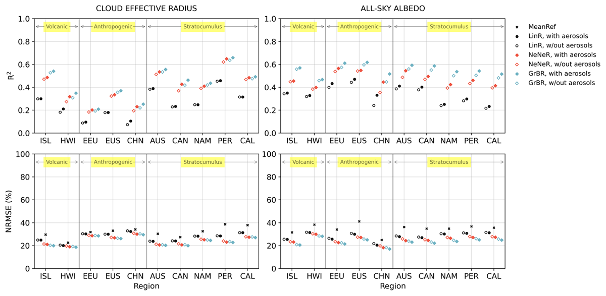
Figure 3
Model evaluation comparing R2 and normalised RMSE scores for NeNeR (red) and GrBR (blue) with a simple linear regression (black circles) and a mean reference model (black cross) for the two response variables reff (left) and all-sky albedo (right). Filled markers represent models with aerosols included and empty markers are models excluding aerosols. Regions are grouped according to their respective category.
3.2 Adding aerosol information
With aerosol information (AOD, SO2 and SO4) added to the meteorological input and air mass information, the R2 for the ten regions ranges from 0.21 to 0.66, with an average of 0.43 further enhancing the skill of the model slightly. This is shown in column ‘ERA + air mass + aerosol’ in Table 4. The improvement in score with addition of aerosol information is smaller than the improvement due to inclusion of AMO and ztop, see Section 3.1. Averaged over the ten regions, the improvement in skill from adding aerosol information is 7%.
For comparison, adding aerosol information to the reference model, without AMO and ztop, results in R2 values from 0.18 to 0.62, with an average of 0.40, also shown in Table 4, column ‘ERA+aerosol’. This corresponds to an improvement in average skill of 9% over the 10 regions.
Figure 3 summarises and compares the coefficient of determination (R2, upper panels) and the normalised root mean squared error (NRMSE, lower panels) of the NeNeR and the GrBR models against the linear regression and a mean reference model. This illustrates that the two machine learning methods are comparable, and that they both perform better than the linear regression model. Further, models generally perform slightly better when aerosol information is included among the predictors, but the improvement is often small and there is no clear pattern between regions or categories in degree of improvement. The greatest difference in comparing the model scores with and without aerosol information included can be seen in the regions HWI, CHN and CAN. The difference in relative error is also small.
The performance of the GrBR is very similar to that of the NeNeR. In the cases with a difference in the score, the GrBR models score better than the NeNeR models. This suggests that the GrBR is more sensitive to hyperparameter tuning than the NeNeR since the NeNeR scored better when default parameter settings were used (cf. Supplementary Information, Figure A.1). Tuning the hyperparameters of the GrBR improved the performance more than could be achieved for NeNeR. However it should be mentioned that the NeNeR model generalizes the data better, meaning that the difference in training score/error and test score/error is less for NeNeR, while the GrBG tends more to overfitting the data. Calculating the model results is also quicker with NeNeR, with a 2–10 faster calculation process in the different regions, than with the GrBR method.
3.3 Predicting albedo
While the microphysical cloud response to changes in aerosol burden are on droplet size and number, the effect on radiation and radiative forcing acts via the reflectivity of the cloud, and its influence on total albedo. As a further test of to what degree radiative forcing due to aerosol-cloud and aerosol-radiation interaction can be predicted based on large amounts of meteorological data, the GrBR and the NeNeR models were also trained on the output variable albedo. For comparability, the same hyperparameter settings were used as for the predictand reff. The results are shown in the right panels of Figure 3. Compared to the prediction of reff, the prediction of albedo yields higher scores for most regions, particularly the anthropogenically influenced regions EEU, EUS and CHN. For some regions (particularly PER) the scores for predicting albedo are lower than those for reff.
The difference in performance between GrBR and NeNeR is greater for the albedo prediction, with the GrBR for all regions producing higher R2 and lower NRMSE, and for all cases the machine learning models here too perform better than a simple linear regression, that in turn performs better than the reference mean prediction.
As in the case of reff, the R2 skill of the model predicting albedo improves most with inclusion of air mass information (average of 28% for the ten regions) and further improves somewhat with inclusion of aerosol information (by an average of 6%).
3.4 Individual parameter dependencies
3.4.1 Relative importance of aerosol, air mass and meteorological parameters
AOD and ztop in some specific regions show high relative importance for the GrBR models, but overall meteorological input variables dominate the relative feature importance, and air mass and aerosol related variables are lower ranked. Rank here refers to the place of this variable in a sorted list of permutation feature dependence for all input variables, see Figure 4. In particular low-level temperature (T1000) ranks high (among the top five) in all regions, but also higher altitude temperature, as well as geopotential height and to some extent low-level relative humidity show high ranks.
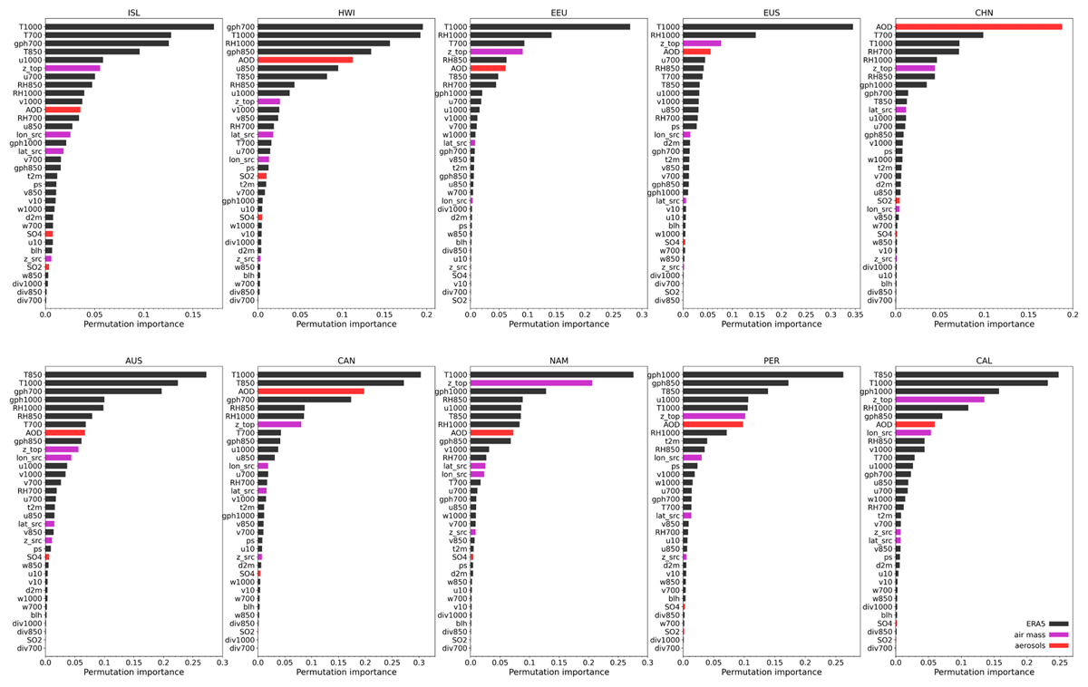
Figure 4
Permutation feature importance for prediction of reff in 10 regions. Meteorological input from ERA5 is marked black, whereas air mass variables (latsrc, lonsrc, zsrc, and ztop) are indicated in magenta, and aerosol variables (AOD, SO2 and SO4) are marked with red. Note the different ranges for the different regions.
The rank of AOD is highest (1) in the CHN region, followed by the CAN region (3). In the other regions AOD is ranked fourth to 11th. The SO2 and SO4 ranks are in all cases among the lowest half out of the 34 parameters. Feature importance for all variables and all regions is shown in Figure 4, and rank for AOD specifically, is listed in Table 5.
Table 5
Mean values of AOD for the ten study regions, and direction of AOD impact on predicted reff (Negative (–) indicating cases where reff is smaller for higher aerosol burden, as expected from Twomey theory, and vice versa.). Feature importance rank of AOD, SO2 and SO4 respectively, out of 34.
| REGION | MEAN AOD | SIGN | RANK AOD | RANK SO2 | RANK SO4 |
|---|---|---|---|---|---|
| ISL | 0.140 | –/+ | 11 | 30 | 26 |
| HWI | 0.133 | – | 5 | 19 | 24 |
| EEU | 0.215 | + | 6 | 34 | 31 |
| EUS | 0.179 | –/+ | 4 | 33 | 27 |
| CHN | 0.636 | + | 1 | 22 | 26 |
| AUS | 0.094 | – | 8 | 33 | 23 |
| CAN | 0.213 | –/+ | 3 | 32 | 25 |
| NAM | 0.236 | –/+ | 8 | 33 | 23 |
| PER | 0.106 | – | 7 | 32 | 29 |
| CAL | 0.111 | –/+ | 7 | 33 | 31 |
For the model predicting top-of-atmosphere albedo, ztop becomes more important, and is among the top-four ranked input variables for all regions, and top ranked for six of the ten models, with greater ztop associated with higher albedo (not shown).
3.4.2 Partial dependence on aerosol and air mass origin parameters
Based on the GrBR analysis, partial dependence plots can provide further insight into the effect of individual variables, or the combination of two variables, on the prediction of the response variable. We present here partial dependence of reff on two aerosol-related input variables (AOD and SO2, Figure 6), as well as on two AMO-related input variables (latsrc and lonsrc, Figure 5).
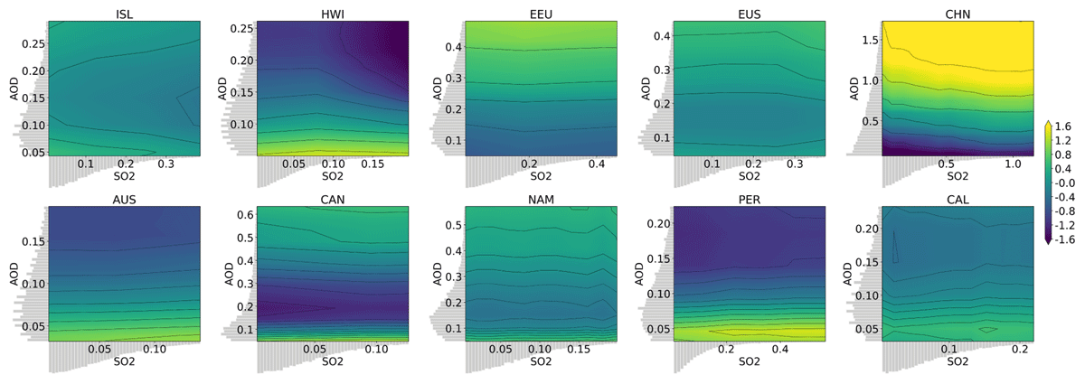
Figure 5
reff dependence on air mass source region (longitude and latitude anomalies) for all ten regions, outlined by white boxes. Grey shading indicates relative distribution of longitude and latitude origin values. The discontinuity at 0° longitude is due to the model being trained on longitudes from 0° to 360° rather than –180° to 180°.
Figure 6
reff (colour and contours) dependence on aerosols (AOD and SO2 anomalies) for all ten regions. Grey shading indicates relative distribution of AOD and SO2 values.
Figure 5 shows that for the stratocumulus regions (AUS, CAN, NAM, PER, CAL), reff generally decreases with increasing (i.e. more easterly) source longitude, whereas the dependence on source latitude is weaker, consistent with more continental air masses coinciding with smaller droplets. The data density information indicates that compared to the other Sc-regions, the PER region more rarely experiences off-shore flow, and that the westerly winds are comparatively strong in the AUS region, with more data points with source region far to the west, for the same 5-day length of trajectories. For the CAN region, the most frequently occurring back-trajectory origin is slightly east of the target region, but for the other Sc-regions westerly or local AMO is most common.
For the two volcanic regions, the ISL region experiences mainly strong westerly flow (Figure 5) and reff is largest for air coming from the North West, and smallest for flow from the South East; the HWI region shows an AMO distribution shifted towards the east of the target region, and the droplet size gradient is mainly in the north-south direction, with reff increasing with increasing latsrc.
For the CHN region, the gradient is also most prominent in the north-south direction, with reff increasing with increasing latitude of AMO. For EEU the dependence on AMO is weak, but reff tends to decrease with increasing latsrc. For the third anthropogenically influenced region (EUS) the pattern is rather one of decreasing reff with decreasing lonsrc, again in general agreement with continental and polluted flow coinciding with smaller droplets.
Note that because the models were trained on longitude ranges from 0° to 360° there is a discontinuity at 0° longitude in these partial dependence plots shown for the range –180° to 180°. The models will learn similar impact strength from the highest and the lowest end of the input range, which especially when occurring at low data density, leads to uncertainty in the determination of partial dependence.
For dependence on aerosol (Figure 6), all regions show a weak dependence on SO2, as expected from the low feature importance. The dependence on AOD is greater, but not consistent across all regions. In the stratocumulus regions, the general decrease in reff with increasing AOD, which might be expected from Twomey theory, is evident. In some of these regions (CAN, NAM) there is a tendency towards the opposite direction at high AOD values (above 0.15–0.2), but the data density is comparatively low in those ranges, meaning both that those cases are rare, and that the model has less data to train on. Similarly for the volcanic regions, ISL and HWI, reff decreases with increasing AOD for the ranges of most prevalent AOD values, and there is indication, particularly for ISL, of a reversal at high AOD values (0.15–0.2), but here too there is not enough data for a reliable interpretation of the data in this range at the tail of the AOD distribution. For the polluted industrial regions, EUS shows the expected pattern of decreasing reff with increasing AOD up to a limit around 0.15 where the gradient reverses, but for CHN, and EEU the dependence is rather clearly of the opposite sign.
The sign of dependence of reff on AOD is also summarised in Table 5, for all regions.
4 Discussion
We have presented a machine learning approach to studying impact of aerosol amount on cloud properties. GrBR models are trained on both meteorological and aerosol data to predict cloud droplet effective radius over 10 regions.
We show that it is possible to predict this cloud microphysical parameter based on large scale meteorological variables only, with some skill (R2 mean 0.41, range 0.19 to 0.64 across regions). The explained variance by the model is on average less than 50%, and there are many reasons to expect discrepancies between the model-predicted and observational values, including the imperfect synchronisation of reanalysis and satellite retrieval in time and space, as well as errors in the model and the retrievals, and without accounting for variations in updraft, supersaturation, size distribution and composition of aerosol, nothing but a crude estimate of cloud characteristics can be expected.
Although the relative error of the GrBR model is fairly large (20–30%) it still performs better than a reference model which always predicts the climatological mean value of the dataset, as well as a traditional linear regression model. Applying a NeNeR model gives very limited improvement in performance. Andersen et al. (2017) who used a similar method (artificial neural network) to predict cloud droplet radius and other cloud properties from reanalysis and satellite data, achieve a somewhat better median performance, but with very large spread across the globe, and with the difference that their model operates on monthly mean scale, rather than on daily resolved data.
The models that are also given information of the AOD have a somewhat better overall score than the models that are only given meteorological information. This suggests that AOD has an impact in determining reff, but the model improvement is small (R2 range 0.21 to 0.66 across regions, with an average of 0.43, only 7% higher than the case with meteorology and air mass information).
Among the selected region classes, the model skill is overall best in the stratocumulus regions, and poorest in the anthropogenically influenced regions. The degree of improvement of the model with aerosol information inclusion does not vary consistently between region types.
The skill of prediction of albedo is somewhat higher than that of reff, bringing the R2 for all regions above 0.4. The improvement in model skill with inclusion of aerosol information is small for albedo prediction as well, although in this case it is less of a limitation that AOD can only be retrieved for cloud-free pixels. In the case of reff prediction, it should be noted that the aerosol information can not be measured simultaneous to the cloud properties, but will rather represent nearby surrounding conditions.
The relative importance of each parameter is also studied. Since the machine learning model used is built on decision trees, the feature importance for each parameter for the different regions is easily determined. It is shown that the importance of AOD varies between the regions, but it ranks among the five most important parameters only in four out of the 10 regions. Hence, although there is a physical relation between aerosol and reff, the quantification of AOD is of limited importance to the prediction of reff.
These results are in qualitative agreement with previous studies on coarser temporal and spatial resolution, using other machine learning models; Andersen et al. (2017) who found aerosol to be a weaker predictor for droplet size and cloud amount than several meteorological measures including lower tropospheric stability, and Fuchs et al. (2018) who found meteorological parameters such as lower tropospheric stability, boundary-layer and surface wind parameters to be most important for reff and cloud fraction in most sub-regions of a stratocumulus-dominated area, even during biomass burning season.
Parameters that are consistently ranked high by the models are primarily temperature and geopotential height and to some extent relative humidity. These and the other input parameters can all be related to actual processes controlling cloud formation and properties, such as vertical motion or advection of air across gradients of temperature or humidity, turbulence from instability or shear, and strength of mixing and entrainment at top of boundary layer, or weather systems and accompanying cloud and precipitation patterns. Although pointing at the temperature at 1000 hPa as the single best predictor, in consistency with previous studies finding sea surface temperature to be the main cloud controlling factor (Myers et al. 2021, Ceppi and Nowack 2021, e.g.) our results do not motivate reduction to one or a few parameters, rather they indicate that the full atmospheric state is helpful for determining the cloud properties.
SO2 and SO4 are ranked among the least important parameters for all of the regions. For SO2, this may be partly due to the OMI data being noisy, and in pre-processing cut off at 0, and averaged over time to account for poor coverage. It may also be due to the fact that the SO2 is a short lived aerosol precursor that is not necessarily limiting for sulfate production, and is therefore not a reliable parameter for the model to base its predictions on. We note that Andersen et al. (2023) also found cloud radiative effects to be less sensitive to reanalysis sulfate than satellite derived AOD or aerosol index. The low feature importance of SO2 as well as SO4 are more unexpected given their demonstrated predictive power over variability in droplet number concentration and size, in McCoy et al (2018) and Wall et al. (2022) respectively. They, however, show co-variation with regional mean scale trends on monthly to decadal time scale, which doesn’t necessarily imply strong control on the short-term variability, and apparently is not picked up by the current model. Furthermore, although reff and droplet number concentration are negatively correlated at fixed cloud water amount, compensating variations in liquid water path may interfere with that relation, and a good predictor of droplet number is not by necessity a good predictor of reff.
Notably, the two regions where AOD ranks the highest in feature importance (CHN and CAN) are also the regions that coincide with higher levels of dust aerosol than the others (Tian et al. 2023, Song et al. 2021, e.g.), and for both these regions, the partial dependence on AMO suggests backward trajectories from nearby dust sources (South-West for CHN and East for CAN) are associated with smaller reff. Similar to the CAN region, all Sc-regions show patterns where more continental air flow is associated with smaller reff.
In some cases, although the influence of AOD on the model prediction of reff is small, its direction is consistent with what is expected from theory, inasmuch as larger AOD values cause the model to predict smaller values of reff. There are other cases where the dependence tends to be reversed at higher values of AOD (ISL, EUS, CAN, NAM, CAL). Even though a reversal in gradient is not expected from theory, it is known that the Twomey effect, or the cloud albedo susceptibility to changes in droplet number concentration, is greater in pristine environments and levels off in more polluted conditions Carslaw et al. (2013). Liu et al. (2017) have showed similar nonlinear behaviour of reff dependence on AOD, albeit with a reversal at even higher AOD values, ascribing the effect to competition for water vapour in highly polluted environments, favouring growth of larger droplets and evaporation of smaller ones, as also discussed by Feingold et al. (2001).
Importantly, though, for these regions, the high AOD ranges at which the indicated reversal of the gradient occurs are quite infrequently occurring, and the dominant signal also for these regions is that of reduced droplet size with increasing AOD.
However, for two regions; most notably CHN where AOD actually has a high feature importance, but also EEU, the AOD variation has the opposite effect for the entire sampled AOD range. Although contrary to the expected Twomey-relation, these results are in agreement with earlier findings: In Andersen et al. (2017) and Andersen et al. (2023) the sensitivity of cloud properties to aerosol is found to be negative on near-global scale, but the geographical distributions nevertheless display variation that confirm the fully or partially reversed relations we find for the EEU, EUS, CHN, CAN, and NAM regions. Andersen et al. (2023) also show that the sensitivity patterns and magnitudes are very similar for AOD and aerosol index. Myhre et al. (2007) attributed positive dependence of satellite derived reff on AOD in regions corresponding to EEU to coinciding decreases in cloud top pressure. Southeastern Asia, where the CHN region is located is further a region where several studies, for instance Yuan et al. (2008), Tang et al. (2014), Wang et al. (2014), Ma et al. (2018), have found positive correlations between AOD or aerosol index and droplet size, particularly over land. While Grandey and Stier (2010) showed that data aggregation to large land regions can result in spurious positive correlations between AOD and droplet size, Jia et al. (2019) discuss the plausibility of positive correlations between AOD and reff, over land areas, suggesting both artificial effects (retrieval biases of both cloud and aerosol), and physical reasons (primarily enhanced entrainment mixing) for its occurrence.
One contributing reason for the increase in droplet size with increasing AOD may be relative humidity effects on the AOD retrieval and estimated relation with cloud properties, with hygroscopic growth of aerosols, rather than aerosol concentration per se, causing high AOD (Myhre et al. 2007, Chand et al. 2012, Altaratz et al. 2013, e.g.).
Since stronger dust signature of the air seems to correlate with smaller droplet size in the CHN region, while the AOD-dependence in general has the opposite sign, it is also possible that AOD in this region is influenced by other less CCN-prone aerosols, such as freshly emitted black carbon (Bond et al. 2013).
Also e.g. Bender et al. (2016), Douglas and L’Ecuyer (2019), Stevens and Feingold (2009) discuss situations in which cloud brightening with increasing aerosol loading is not necessarily manifest as expected from cloud brightening, e.g. due to aerosol vertical distribution, cloud thickness and ambient stability.
Finally, we note again, that the fact that cloud liquid water path is not controlled for may interfere with the results. The droplet size is determined not only by the number of droplets, but also by the amount of water in the cloud, and it is possible that even if the high aerosol content leads to more droplets, the decrease in droplet size is offset by increased water content, that is not controlled for in this study.
5 Conclusions
We have shown that a simple machine learning model (gradient boosting regression, GrBR) can be constructed, that with meteorological and air mass origin input data can with some skill predict cloud microphysical properties, represented by droplet effective radius (reff). The model performs better than a simple linear regression model. Information on aerosol optical depth (AOD) makes the model perform somewhat better, but AOD is in most cases of low relative importance for the model, and the direction of aerosol influence on reff is not consistent. While the model for most regions links greater AOD to smaller reff, at least for the most prevalent AOD ranges, two of the anthropogenically influenced regions show a reversed signal. The model skill is highest in subtropical stratocumulus regions, with mean R2 of 0.5 over Australian, Canarian, Namibian, Peruvian and Californian regions, and lowest in industrial polluted regions, with mean R2 of 0.3 for regions over Eastern China, Eastern US and Eastern Europe. Information on boundary layer sulfur dioxide concentration and near-surface sulfate mass, from satellite and reanalysis respectively, has little effect on score and prediction. Other machine learning models (specifically a neural network regression, NeNeR) don’t necessarily perform better than the GrBR. Training the model to predict all-sky albedo gives performance that is somewhat more consistent, and R2 above 0.4 for the GrBR for all regions. The presented method of including and excluding aerosol information in a data driven model, offers a new approach to the challenge of distinguishing aerosol effects on cloud properties, and the results emphasize the role of local meteorology.
Additional File
The additional file for this article can be found as follows:
Supplementary Information
Comparison of different machine learning models. DOI: https://doi.org/10.16993/tellusb.1868.s1
Funding Information
We acknowledge support from the Swedish e-Science Research Centre (SeRC), from the Wenner-Gren foundation, and from the FORCeS project funded by the European Union’s Horizon 2020 programme, Grant Agreement No. 821205. FB thanks the Department of Atmospheric Sciences, University of Washington, Seattle, USA for hosting her sabbatical, where the work was completed. The computations were enabled by resources provided by the National Academic Infrastructure for Supercomputing in Sweden (NAISS) and the Swedish National Infrastructure for Computing (SNIC) at the National Supercomputer Centre (NSC) partially funded by the Swedish Research Council through grant agreements no. 2022-06725 and no. 2018-05973. We further acknowledge the NOAA Air Resources Laboratory (ARL) for the provision of the HYSPLIT transport and dispersion model used in this work.
Competing Interests
The authors have no competing interests to declare.