
1 Introduction
The Southern Ocean is connected to the Pacific, Atlantic, and Indian Oceans, and plays a crucial role in determining the global ocean’s carbon and heat content (e.g., Ferrari et al., 2014; Galbraith and de Lavergne, 2019; Talley et al., 2011). A key feature of the Southern Ocean is the Antarctic Circumpolar Current (ACC), with a thermal wind transport (relative to the sea floor) of around 137 Sv (e.g., Meredith et al., 2011). Understanding the processes that govern the ACC and its sensitivities to changing conditions is is crucial for predicting how the global climate might respond to changes in the atmospheric forcing, ranging from natural variations such as that occurring in past climate (e.g., Scher et al., 2015; Toggweiler, Russel and Carson, 2006; Xing et al., 2022) to anthropogenic signals under projected climate change scenarios (e.g., Fyfe et al., 2007).
There have been ample investigations showing that the existence of the ACC depends on the wind and buoyancy forcing over the Southern Ocean region. Strong westerly winds blow over the Southern Ocean, with the wind stress maximum positioned roughly at 50°S for the present-day setting (Large and Yeager, 2009). These winds drive a northward Ekman transport at the surface, which is balanced by a southward flow at depth (Nikurashin and Vallis, 2012), resulting in upwelling at the southern edge of the ACC and downwelling at the northern edge, driving a meridional overturning circulation. The wind-induced overturning tilts the Southern Ocean isopycnals, creating a strong meridional pressure gradient that, in turn, results in a strong eastward geostrophic current (Rintoul, 2018). On the other hand, atmospheric buoyancy forcing can affect the out-cropping locations of the Southern Ocean isopycnals, which has a consequence on the resulting Southern Ocean stratification profile, and thus the ACC transport via the thermal wind shear relation (e.g., Hogg, 2010; Howard et al., 2015; Hughes and Griffiths, 2006; Klocker et al., 2023).
However, numerous studies have highlighted that transient baroclinic mesoscale eddies and geostrophic flow–topography interactions play a crucial role in the resulting ACC transport and its sensitivity. Both transient baroclinic mesoscale eddies and standing eddies resulting from flow–topography interactions lead to form stress (e.g., Johnson and Bryden, 1989; Masich, Mazloff and Chereskin, 2015, 2018; Stewart, Neumann and Solodoch, 2022; Vallis, 2006; Youngs et al., 2017) thereby induce vertical fluxes of horizontal momentum, impacting the momentum budget and the resulting circulation in the system (e.g., Marshall et al., 2017). For example, the phenomenon of eddy saturation—whereby the ACC transport is largely insensitive to the changes in the wind stress magnitude (e.g., Constantinou and Young, 2017; Constantinou and Hogg, 2019; Hallberg and Gnanadesikan, 2006; Marshall et al., 2017; Munday, Johnson and Marshall, 2013; Straub, 1993)—is argued to result because the eddy component increases with the wind component such that there is complete cancellation of the two competing effects, leading to a transport independent of the wind stress magnitude (e.g., Marshall et al., 2017). Whether eddy saturation is observed in numerical models depends critically on how the eddies are represented (e.g., Farneti et al., 2015; Fox-Kemper et al., 2019; Hallberg and Gnanadesikan, 2006; Mak et al., 2017, 2018, 2022a; Munday, Johnson and Marshall, 2013; Toggweiler and Samuels, 1995). In addition, the Southern Ocean is connected to the other ocean basins, and the ACC is not contained solely within the open-channel latitudes of 56°S–58°S (Rintoul, 2018), going as far north as 38°S (Talley et al., 2011) in the southwest Atlantic. The traditional understanding of these northern excursions is through Sverdrup balance, and in order to fully represent Southern Ocean dynamics, eddy-induced downwelling must also be taken into account (e.g., Marshall et al., 2016; Nadeau and Ferrari, 2015). Modelling studies have shown that a significant ACC transport persists even when the wind jet is moved completely north of the channel (e.g., Allison et al., 2010; Marshall et al., 2016; Munday, Johnson and Marshall, 2015), suggesting that the basin can play an important role in ACC dynamics. Furthermore, the presence of a residual meridional overturning circulation (RMOC) can impact the model response (e.g., Howard et al., 2015; Stewart and Hogg, 2017). However, how wind forcing and eddy effects balance in the presence of a basin region and/or an RMOC remains to be thoroughly investigated.
The present work aims at studying how the sensitivity of the ACC transport to changes in wind forcing depends on the RMOC, focusing particularly on the case of a negative RMOC (defined as a poleward above-pycnocline mass flux into the Southern Ocean). The primary motivation for the present work is the results from Mak et al. (2018; 2023) and Youngs, Flierl and Ferrari (2019), where the ACC transport is sometimes observed to decrease with increasing wind forcing; we refer to this phenomenon as negative sensitivity in this work. Mak et al. (2018; 2023) report such a negative sensitivity in their primitive-equation channel model where the diagnosed RMOC is in the negative sense (resulting from the enhanced diffusivity region in the north), not only for the case where eddies are explicitly resolved, but also for a case where an eddy-energy-constrained eddy parameterisation from Marshall et al. (2012) and Mak et al. (2018) is used (see Fig. 1a of Mak et al. 2018, green and red curves). Youngs, Flierl and Ferrari (2019) report on a negative sensitivity in a two-layer quasi-geostrophic system with an imposed negative RMOC (achieved via imposing mass transfers between the layers), but not when the imposed RMOC is positive or zero (their Fig. 4, solid purple lines). Although the negative RMOC scenario (corresponding to a negative in Fig. 1a later) could be considered unconventional relative to present day scenario, it has been theorised that, over geological timescales, there were certain periods during which North Atlantic Deep Water formation was greatly weakened, and could even have totally collapsed (Rahmstorf, 2002). During such times, an upper cell of the meridional overturning circulation that is reversed compared to the present-day scenario is possible (e.g., Zhang et al., 2022), and there have been works in the paleoclimate literature on related scenarios (e.g., Huber and Nof, 2006; Munday et al., 2024; Sauermilch et al., 2021; Xing et al., 2022).
In this article, we explore the dependence of equilibrium ACC transport on wind forcing (location and magnitude), RMOC direction and the eddy representation in an idealised channel-basin model, with a focus on the conditions required to reproduce negative sensitivity. An idealised channel-basin model is used to fully explore the parameter space in a computationally tractable way, in particular, the dependence of the observed sensitivity on the location of wind forcing (e.g., wind forcing solely over the channel vs. wind forcing solely over the basin). We make a simplifying assumption to exclude flow–topography interaction effects and demonstrate that, with only transient eddy effects, we are able to reproduce negative sensitivity and derive scalings for the underlying process. We use eddy parameterisations to represent the effect of transient eddies, and we primarily focus on the results from the GEOMETRIC eddy parameterisation (e.g., Marshall et al., 2012; Mak et al., 2017), which has been shown to be able to capture the sensitivities of eddy-resolving/permitting primitive equation models (e.g., Mak et al., 2018, 2022a, 2023; Wei, Wang and Mak, 2024). For the present work, we mimic the effects of an RMOC by varying the boundary conditions at the northern part of the basin, where a negative RMOC corresponds to a poleward above-pycnocline mass flux into the system from the model northern boundary, leading to a deepening of the modelled pycnocline, and vice-versa for the case of positive RMOC; such a choice allows for a control of the RMOC sign and strength as a system parameter. We additionally present a numerical methodology that greatly speeds up the relevant computations for the present idealised model, allowing us to explore the parameter space comprehensively for studies of equilibrium sensitivity, with potential adaptations for other paleoclimatology studies such as that of Huber and Nof (2006) and Munday et al. (2024). We should be upfront and say that our presented analysis is perhaps not as theoretically satisfactory as it could be, and can likely be refined and made more comprehensive. Nevertheless, we think the explanations presented support and highlight an interesting mechanism at play in the control of the ACC transport.
The structure of this article is as follows. Section 2 describes the general formulation of the model, the details relating to the eddy parameterisations used for the present work, the exact model setup and numerical implementation details. Section 3 provides the numerical results for the case with wind solely over channel, highlighting the eddy saturation and negative sensitivity phenomenon, with a focus on the negative RMOC setting. Section 4 provides an analysis towards understanding the eddy saturation and negative sensitivity phenomenon, offering a physical rationalisation for the latter. Section 5 presents additional numerical results under different wind forcing regimes to highlight similarities and differences with the control setting. We summarise our results in Section 6.
2 Model Details, Parameterisation Formulation and Numerical Implementation
For the present work, we essentially use the 1.5-layer reduced gravity model of Marshall et al. (2016), with modifications primarily in the prescription of the Gent–McWilliams coefficient , and the imposed boundary condition to independently modify the strength and direction of the RMOC. The 1.5-layer reduced gravity model is a particularly simple setup that supports a wind-driven ACC (e.g., Marshall et al., 2016; Munday et al., 2024), although it does exclude any representation of flow–topography interactions. We first recap the broad details in the model of Marshall et al. (2016), and then proceed to state the relevant modifications implemented in this work.
2.1 Details of model
A 1.5-layer reduced gravity model effectively represents the dynamics above the main pycnocline, with an upper layer thickness denoted by h that varies in space and time, where the density of the upper layer is kept constant. The representation of the buoyancy effects is through a reduced gravity , where denotes the density difference between the layers (e.g., Vallis, 2006). To derive the equation for h, we start from the shallow water equations:
where (1a) is the momentum equation and (1b) is the continuity equation, and is some diabatic forcing term to be specified. The two-dimensional horizontal velocity vector is denoted by u, is the Coriolis parameter under the -plane approximation, with f0 being the value of the Coriolis parameter at the southern end of the model, the rate of change of f along the meridional direction, the unit vector in the vertical direction, and denotes the horizontal gradient operator. The wind stress at the ocean surface is (where we have made the assumption that ). The terms on the right-hand side of (1a) correspond, respectively, to the Coriolis effect, pressure gradient force, wind stress and a friction term. For simplicity, we consider a linear friction term acting on the geostrophic flow, with a constant but small coefficient r, to enforce the no-normal-flow boundary conditions in the presence of along-boundary variations in h (or pressure), following Marshall et al. (2016). The presence of friction is not intended to be a parameterisation of the mean feedback of baroclinic eddies (as a vertical diffusion of momentum, related to the form stress in the geostrophic regime, e.g., Greatbatch and Lamb, 1990), which we will come to shortly. In the present case, the friction terms essentially play a negligible role in the resulting balances except near boundaries of the domain, where it is a crucial component in light of an eddy contribution that will be tapered towards zero as the boundaries are approached to ensure no eddy flux normal to the boundary.
For the present work, we are interested in obtaining the equilibrium state. We consider the regime where the Rossby number is sufficiently small, so that the left-hand side of (1a) may be neglected relative to the terms on the right-hand side (or that we are roughly in the planetary geostrophic regime). We split the variables into a mean and eddy part as and , where overbars represent a Reynolds averaged component, and the primes denote the deviations from that average. We assume the Reynolds averaging operator is such that and , and commutes with derivatives. Taking an average of Eq. (1a) leads to:
where we have assumed that (which requires ) and that the wind stress has no fluctuating part. We further multiply Eq. (2) by , and taking the vertical component of the curl (i.e. ) results in
Under a Reynolds average of Eq. (1b), the terms linear in the eddy components vanish under the averaging procedure. Following the work of Marshall et al. (2016), the Gent–McWilliams parameterisation (Gent and McWilliams, 1990) is invoked; while the parameterisation has the form of a diffusion in h, it is more accurately an eddy-induced transport with eddy-induced velocity (e.g., Gent et al., 1995), and is better described as an eddy-induced velocity coefficient. With this, Eq. (1b) becomes
Substituting Eq. (4) into Eq. (3) and dropping all the overbars then leads to a single equation in terms of the mean scalar variable h, given by
The terms on the right-hand side correspond, respectively, to the eddy term, the geostrophic term, the Ekman term associated with wind forcing, the friction term and a restoring term to be specified. Expanding the divergence term in Eq. (5) results in Eq. (2.4) of Marshall et al. (2016); we leave the present equation in terms of a divergence for the numerical implementation detailed in Sec. 2.3.
To mimic the outcropping of isopycnals at the south, we impose a Dirichlet condition on h at the southern boundary when we numerically solve for Eq. (5), which physically corresponds to an implied mass flux in or out of the system from the northern boundary. In places where we would impose a no-normal-flow boundary condition (denoting n as the outward pointing unit vector normal to the lateral boundary), a domain-integral of Eq. (4) and a use of the divergence theorem would imply that we need ; this will be achieved by tapering to zero as we approach the relevant boundaries when we numerically solve for Eq. (5), and in this instance, the friction term is necessary to support a physical balance (tests show numerical non-convergence if friction is absent; not shown). A more problematic case is for Eq. (3), where a similar procedure leads to
needing to be satisfied everywhere on the domain boundary corresponding to the lateral walls. We will structure the wind stress profile so that at the boundaries, so the third term of Eq. (6) vanishes. No-normal-flow condition then implies we need
to be satisfied locally on the boundaries when we numerically solve for Eq. (5). The condition given by Eq. (7) is that of Eq. (2.3) in Marshall et al. (2016), up to some proportionality factors, and results from enforcing the no-normal-flow conditions in the presence of along-boundary variations in h. At first sight, this boundary condition might be problematic to implement; however, it turns out we can bypass it entirely in our numerical formulation presented in Sec. 2.3.
2.2 GEOMETRIC prescription of the eddy-induced velocity coefficient
From hereon, we deviate from the work of Marshall et al. (2016): we consider different prescriptions of the eddy-induced velocity coefficient . The principal focus here is the GEOMETRIC parameterisation (e.g., Marshall et al., 2012; Mak et al., 2017, 2018), which has been seen to lead to model calculations that demonstrate a negative sensitivity where the circumpolar transport decreases with increasing wind stress, in line with some eddy-rich calculations (Mak et al., 2018; Youngs, Flierl and Ferrari, 2019); see also Fig. 8b in Mak et al. 2023.
The GEOMETRIC parameterisation was originally formulated for systems that are continuously stratified, and here we provide a derivation that is more relevant for shallow water systems. Starting from , the Cauchy–Schwartz inequality (e.g., Evans, 1998) results in
In addition, we have
where and are the eddy potential and eddy kinetic energies per unit mass, and D is the total depth of the ocean. Since the total eddy energy per unit mass , it follows that, using , we have
where we write for ease of reading in later sections; note that this is a vertically integrated quantity and has dimensions . With and assuming that , we obtain
where we have, for simplicity, assumed a uniform gravity wave speed via substituting h with D; this simplification makes the analysis presented in Sec. 4 more concise, and the numerical results display quantitatively robust behaviour whether or not h or D is used (not shown). The non-dimensional variable satisfying can, in principle, vary as a function of space and time, and is normally interpreted to represent an eddy efficiency; for simplicity, we also take it as a constant in this work. We will denote calculations that use Eq. (11) as GEOM.
To close Eq. (11), we need to have information relating to the eddy energy. For this, we follow Mak et al. (2022a) by providing a prognostic equation for the parameterised eddy energy that varies in two-dimensional space. The choice of the exact prognostic eddy energy equation can be seen as a modelling choice (constrained by theory where appropriate), which in this work we take to be
The source term of the present equation mirrors the loss of available potential energy resulting from the eddy-induced advection from Eq. (5). Following previous works (e.g., Mak et al., 2017, 2018, 2022a, 2022b, 2023; Marshall et al., 2017), we take the dissipation of eddy energy to be linear and governed by a constant dissipation time-scale . This choice is made for simplicity, although analyses suggest that a dominant sink of eddy energy dissipation in the ocean may be non-propagating form drag (e.g., Klymak, 2018; Klymak et al., 2021) leading to linear dissipation of eddy energy. The presence of maintains a minimum eddy energy level (e.g., from sub-grid processes) and also serves to damp large variations in the eddy energy as the iterations proceed (Maddison et al., 2025). We assume that there are some non-local effects represented by advection (e.g., baroclinic instability feeding back onto the mean flow as it is being swept downstream by the mean flow), and here, we include advective effects from both a mean geostrophic velocity and westward propagation at the long Rossby phase speed. The choice of advective terms is motivated by similar choices taken in ocean general circulation models to reproduce a semi-realistic eddy energy field that is comparable to higher-resolution models and observational data (e.g., Mak et al., 2022a, b), but it is ultimately a modelling choice. An eddy energy diffusion term is included primarily as a numerical stabiliser. We enforce the lateral boundary condition so that there are no boundary contributions to the eddy energy.
For comparison purposes, we consider two other prescriptions of . One is the case where , for comparison to the previous work of Marshall et al. (2016). The other is a mixing length-type prescription that also uses eddy energy information. The mixing length prescription considers (noting that E as defined is the domain integrated eddy energy), where L is some length-scale, taken here to be the Rossby deformation radius given by (cf. Jansen et al., 2019; Mak et al., 2017); we have also assumed uniform gravity wave speed to be consistent with the approximations made in GEOM. Calculations using these two prescriptions will be denoted CONST and ML, respectively; only GEOM and ML calculations solve Eq. (12).
2.3 Numerical implementation
We numerically solve for the equilibrium solution associated with Eq. (5) and Eq. (12), subject to appropriate boundary conditions detailed previously. For the model set up, we follow the specifications of Marshall et al. (2016). The model spans in the zonal co-ordinate x, in the meridional co-ordinate y, and we take z to denote the vertical co-ordinate. Figure 1a provides a schematic of the model.
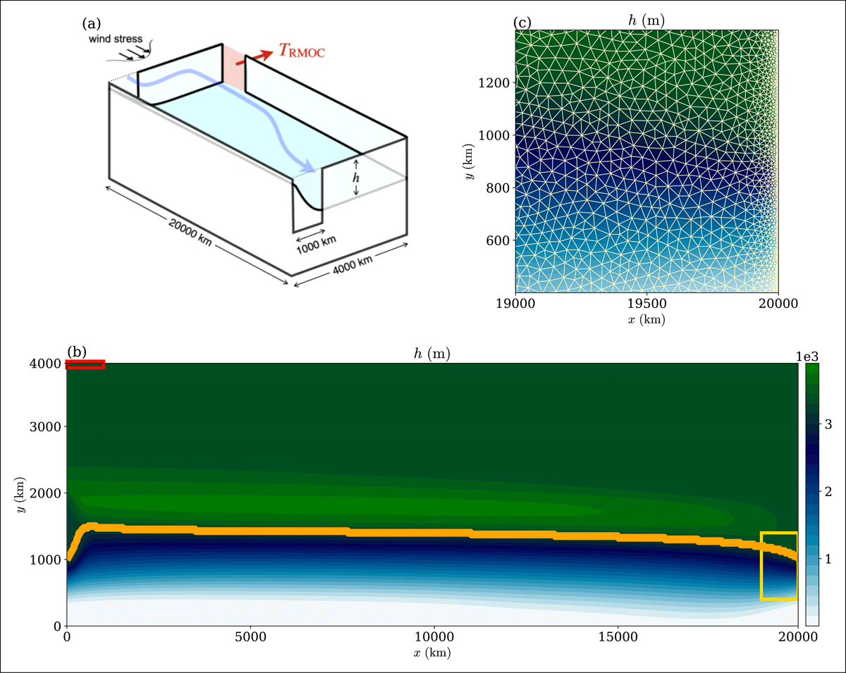
Figure 1
(a) A schematic outlining the geometry of the model, with the layer interface depicted in light blue. The blue arrow represents a streamline of the flow, and the red arrow represents a prescribed outflow as defined in (18). (b) The model pycnocline depth h of a sample equilibrium state for GEOM for a calculation with wind over both the channel and basin region (W02, with , ), for , . The orange contour represents a streamline originating from the northern end of the model Drake passage located at (x,y) = () km, roughly denoting the northern boundary of the modelled ACC. The region enclosed in red denotes the location where the boundary condition of is applied, and the region enclosed in yellow denotes the section of the domain shown in (c). (c) The section of the domain denoted by the yellow region in (b), shown with the numerical unstructured mesh overlaid (light yellow).
There are several numerical methodologies one could use. The previous works of Gill (1968) and Marshall et al. (2016) effectively time-step into the equilibrium (the latter work using a multi-grid method to speed up the process). In this work, we directly solve for the equilibrium state: we leverage existing computational frameworks with in-built solvers for the steady-state problem at hand. One such framework is that of FEniCS (e.g., Alnæs et al., 2015), which is a platform using the finite element discretisation with automatic code generation capabilities, and is particularly convenient for solving problems of the type considered in this work. To use FEniCS, we derive what is known as the weak form of the equations, where the equations are in an integral form, and we seek solutions that satisfy the equations in the weak or averaged sense, in this case over an element (cf. strong form, where we seek for solutions that satisfy the equations in a point-wise or the strong sense). The weak form of the equations is implemented at a high level in Python, via what is known as the Unified Form Language (e.g., Alnæs et al., 2014). The code is then passed onto the FEniCS engine that leads to compiled low-level code in C++ solving for the resulting variational problem, leveraging a wide range of existing solvers for such problems. An example of the Python code demonstrating the procedure is given in Figure 2, where F is related to the weak form (lines 13–20), and we simply ask for it to be solved with some solver parameters (line 22).
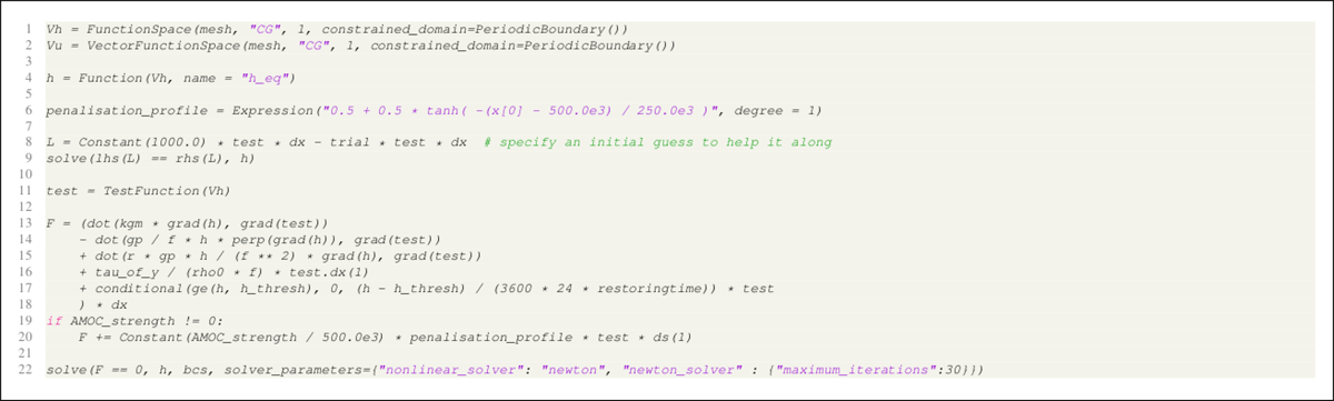
Figure 2
FEniCS code for solving the steady-state equation in its weak form as outlined in Eq. (14).
To obtain the weak form, we return first to Eq. (5) and (12), multiplying the relevant equations with a scalar test function (which is assumed to be as many times differentiable as necessary), and we perform integration by parts and invoke boundary conditions as appropriate. Starting first with Eq. (5), multiplying both sides by and integrating over the domain leads to
where is the area element. If we perform an integration by parts, the boundary contributions from the first integral all vanish by the no-normal-flow condition (see text surrounding Eq. 6), resulting in
where denotes the boundary of , and is the line element corresponding to the boundary of area element . Here, is some prescribed boundary velocity representing a boundary in/outflow. Since the location of in/outflow will be situated at the northern boundary, , and we define the RMOC strength to be . Equation (14) is essentially what is given in Figure 2 (lines 13–20) under the FEniCS framework. To mimic the outcropping at the Southern part of the domain, we enforce a Dirichlet condition on the Southern boundary.
By a similar procedure, the weak form of Eq. (12) becomes (noting that we imposed no normal flow conditions and on boundaries so that there are no boundary contributions to the eddy energy)
For the present model, we construct an unstructured finite element mesh using the Gmsh software (Geuzaine and Remacle, 2009). The mesh elements are triangular elements, with a characteristic spacing of 50 km in the domain interior, gradually refining to elements with a characteristic grid spacing of 1.25 km near the meridional boundaries, and 5 km near the zonal boundaries, over a transition region of 200 km from the boundaries. Any periodic boundary conditions present in the model geometry are imposed as boundary conditions, as opposed to a connectivity in the elements, e.g., forming a cylinder with a wall. The domain contains a total of 1,71,906 elements, and a visualisation of the mesh is shown in Figure 1c. We take the basis function on the elements as CG1 (i.e., first-order Lagrange polynomials), since the weak forms in Eqs. (14) and (15) only demand our solutions to be once weakly differentiable (cf. the strong form, which requires second derivatives to exist).
To complete the specification, we take the restoring term to be
where m and days is the characteristic restoring timescale that measures the strength of restoring, which serves to maintain a minimum layer thickness in the cases where the dynamics thin the pycnocline sufficiently (as an addition of mass, which occurs only when is greater than or equal to zero and in isolated regions of space). Wind stress is taken to be ( the unit vector pointing in the zonal direction), with
where ys and yn are the southern and northern limits of the wind stress, and is the maximum wind stress magnitude. In this study, we report results from three representative wind forcing profiles: one where the wind is only over the channel ( km and km, denoted W01), one where the wind is over both the channel and the basin ( km and km, denoted W02) and one where it is only over the basin ( km and km, denoted W23), following the naming convention of Marshall et al. (2016). Other cases have been considered, but the chosen three cases are representative examples relating to our investigation here.
To represent the effect of an RMOC in this model, we take
where km and km relates to the width of the in/outflow region, and A is a constant chosen so that for some specified . A negative value corresponds to , i.e., a poleward above-pycnocline flow into the domain. Instead of imposing an extra in/outflow boundary condition, a possible alternative is to consider an equivalent forcing/damping in h over an analogous region. Both approaches have been considered in this work and lead to qualitatively similar results; all results presented in this work were computed via specifying an in/outflow boundary condition given in Eq. (18).
To solve for the coupled problem of Eqs. (14) and (15), we solve Eq. (14) first, then Eq. (15), and count that as one iteration, rather than solving both at the same time (i.e., a low-order fixed-point iteration). For GEOM, when updating with Eq. (11), we impose a lower bound of for the local value of to prevent the value of from becoming too large when is too small. We have confirmed that the present methodology is able to reproduce the entirety of the results of Marshall et al. (2016) (the CONST case with zero ; not shown). In terms of performance, the present code can solve for the equilibrium solution in the order of minutes when run on a commercial laptop computer (Macbook with Intel CPU, with calculations performed on a single CPU), compared to, for example, the multi-grid method of Marshall et al. (2016) that can take up to a few hours to reach equilibrium for the CONST calculations, and up to a few days for the GEOM calculations. The speed up in performance is particularly beneficial for our investigation over the parameter space. Table 1 summarises the model parameter values of the set of calculations reported in this work. A relatively large range of is chosen in anticipation of the scaling analysis to be performed. While there is freedom to tune the parameterisations such as , , and , the qualitative results are insensitive to their exact choices, and the documented values were empirically chosen following previous works (e.g., Marshall et al., 2016) or from numerical considerations (e.g., or too large leads to solution convergence issues when is positive in the low wind forcing regime).
Table 1
A list of the relevant constants and parameters for the calculations reported in this work.
| PARAMETERS | VALUE | UNITS | DESCRIPTION |
|---|---|---|---|
| Lx | 20,000 | km | Zonal width of the domain |
| Ly | 4,000 | km | Meridional width of the domain |
| gr | 0.01 | m s-2 | Reduced gravity |
| 1,027 | kg m-3 | Density of the upper layer | |
| f0 | s-1 | Coriolis parameter at the southern end of the domain | |
| m | |||
| r | s-1 | Linear drag coefficient | |
| D | 5,000 | m | Total depth of the ocean |
| 0.03 | Eddy efficiency (GEOM) | ||
| s-1 | Eddy energy dissipation coefficient | ||
| 1,000 | Eddy energy diffusion coefficient | ||
| 1,000 | Gent–McWilliams eddy coefficient (CONST) | ||
| 0.063 | Eddy efficiency (ML) | ||
| E0 | 10.0 | Minimum eddy energy | |
| 0.05, 0.1, 0.2, 0.4, 0.6, 0.8, 1.0, | N m-2 | Maximum surface wind stress | |
| 1.2, 1.5, 2.0, 2.5, 3.0, 3.5, 4.0 | |||
| (W01) | 0, 1,000 | km | Southern & northern boundaries of wind stress (W01) |
| (W02) | 0, 2,000 | km | Southern & northern boundaries of wind stress (W02) |
| (W23) | 2,000, 3,000 | km | Southern & northern boundaries of wind stress (W23) |
3 W01 Case: Wind Forcing Solely Over Channel
We first present results in the case where the wind forcing is solely over the re-entrant channel (W01, where there is no geostrophic contribution leading to Sverdrup balance-like regimes in the present 1.5-layer reduced gravity setting; e.g., Johnson and Bryden 1989), highlighting features of interest that motivate the subsequent analysis. The primary focus will be on the GEOM calculations, where the eddy-induced velocity coefficient is described by the GEOM scaling in Eq. (11), for different choices of .
A typical equilibrium solution in the W01 calculation is one where the fluid layer is thin in the southern part of the channel (as a result of the imposed Dirichlet boundary condition to mimic the outcropping) and the edge of the model ACC coincides with the model Drake passage latitude (not shown, but cf. Figure 1a). We define the (geostrophic) transport streamfunction such that
which is the contribution coming from the geostrophic flow and the eddy-induced velocity, respectively, on the right-hand side. The transport streamfunction here may be obtained by integrating in the meridional direction starting with from the northern boundary. A quantity of interest in this work is the model ACC transport, which we diagnose as the value of at and at the south-western corner of the domain, consistent with the approach taken in Marshall et al. (2016). We show in Figure 3 the diagnosed ACC transport across the GEOM, ML and CONST calculations for a rather large variation in the peak wind-stress and different choices of to comprehensively explore the sensitivities of the model.
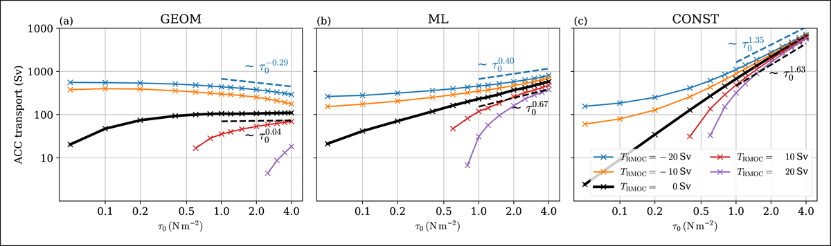
Figure 3
Diagnosed ACC transport for a case where the wind is completely over the re-entrant channel (W01), for different values of and on a logarithmic scale on both axes, for (a) GEOM, (b) ML and (c) CONST. When , at low winds the transport goes to zero, and there is no equilibrium solution (since no mass balance is possible in those cases). The data scalings shown as black dashed line and blue dashed line are diagnosed via a regression over the indicated data range corresponding to the length of the dashed lines using data from the and calculations, respectively.
For zero (the black lines), among the GEOM, ML and CONST calculations, only the GEOM calculations show evidence of eddy saturation, i.e., an ACC transport that is weakly dependent on the wind forcing at large magnitudes of wind forcing, in line with previous results from studies involving GEOMETRIC. On the other hand, the ML and CONST display an increase of transport with wind stress; the diagnosed scalings are and , respectively, in the large wind forcing regime ().
For negative , we see that only GEOM shows the negative sensitivity where the transport decreases with increases in wind forcing. The diagnosed scaling is for in the large wind forcing regime (). All other cases result in an increasing circumpolar transport with increasing wind forcing.
As a first step towards investigating the mechanisms at play, we compute the meridional momentum contributions to highlight differences in the momentum balances between the set of calculations. Upon solving for the scalar field h, we can diagnose the relevant terms in Eq. (5). If we consider the zonally integrated meridional component of the momentum balance, we would have
where
with given by (17), where we have assumed that the integral of is negligible. Note that after integrating, and is non-zero in the domain but vanishes over the circumpolar channel by the periodic boundary condition. The integrals are over the zonal extent of the model domain, and the quantities in (21) represent the net northward volume transport as a function of latitude y.
Figure 4 shows a set of diagnostics relating to the meridional momentum balance. Starting first with the case with zero in Figure 4a–c for a rather large wind forcing case of , we note that all values are essentially zero outside the re-entrant channel, and the dominant balance is between the Ekman forcing (which is fixed once the wind forcing is chosen) and the eddy forcing, with minor but important variations between the GEOM, ML and CONST calculations. In the present channel case, the geostrophic contribution is zero by definition, and the secondary contributions are from friction contributions (cf. Fig. 10 of Marshall et al. 2016). The diminished presence of the term in GEOM would be consistent with the fact that the described by GEOM leads to an eddy component that can entirely compensate for the wind input for sufficiently large wind forcing, i.e., eddy saturation. The same cannot be said of the ML and CONST cases, where the frictional component takes up the residual (which is larger to compensate for the weaker eddy component in balancing the wind input), leading to a change in the resulting equilibrium solution that has a different sensitivity to changes in wind forcing.
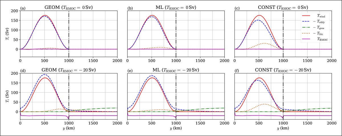
Figure 4
Diagnostic relating to momentum balance for a case where the wind is completely over the re-entrant channel (W01), showing net northward volume transports for a representative case with peak wind stress for (top row) and (bottom row) , for (a,d) GEOM, (b,e) ML and (c,f) CONST. The quantities , and are shown with the opposite sign (dashed lines) to enable easier comparison of magnitudes and distributions. The vertical dashed-dot grey line denotes the model Drake passage separating the channel region and the basin region.
In Figure 4d–f, we show the same momentum balance but for a negative case (, to mean a poleward above-pycnocline mass flux into the system from the model northern boundary). Within the channel region, most of projects onto the eddy component for GEOM and ML (Figure 4d,e), with some of it taken up by the friction component. In both GEOM and ML, the eddy component now supersedes the wind-forcing component everywhere. However, note that GEOM displays negative sensitivity and ML does not (Figure 3a,b). The inconsistency seems to suggest the mechanism at play may be more subtle than one based on broad balances.
Note also that, in the basin region, the presence of the residual projects onto a small eddy term (because of a non-zero as a result of the inflow boundary condition and diffusive-like behaviour of the eddy term ; cf. Figure 5a) and onto the geostrophic component, while friction contributions remain negligible (except near boundaries where the eddy terms are tapered to zero). The non-zero geostrophic term implies that there is some flow driven by a negative . The deepening effect of the pycnocline from a negative RMOC, together with the fixed outcropping, results in the thickness h increasing as we move northwards, and a geostrophic flow associated with the gradient in h must result via geostrophic balance.
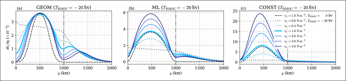
Figure 5
The zonally averaged profiles of the W01 case (wind forcing only over the channel) for (a) GEOM, (b) ML and (c) CONST. The data plotted here are the profiles where there is no wind but fixed negative RMOC ( and ; grey dotted), only wind but no RMOC ( and ; black dashed), and intermediate profiles varying at fixed negative RMOC (; darker blue with increasing ). The vertical dashed-dot grey line denotes the model Drake passage separating the channel region and the basin region.
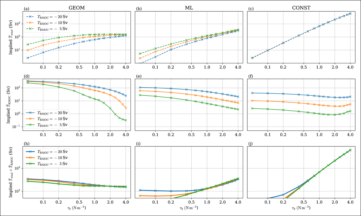
Figure 6
The implied ACC transports from Eq. (32) from the optimisation calculation stated in Eq. (31) for the wind solely over the re-entrant channel (W01). (Top row) . (Middle row) . (Bottom row) , to be compared with results in Figure 3. See Figures A.1 and 5 for samples of the respective definitions of the basis patterns and .
4 Analysis Relating to Eddy Saturation and Negative Sensitivity
It should be noted that the negative sensitivity observed arises from a combination of the wind forcing and the imposed . The momentum budget decomposition (e.g., Figure 4) suggests that, while the eddy contributions surely play an important role, the mechanism is likely subtle and depends on the solution structure, requiring an approach beyond a coarse scaling argument. We provide in this section a mechanistic explanation and some scaling arguments to rationalise the negative sensitivity phenomenon.
4.1 The zero RMOC case, and eddy saturation
It turns out to be informative to consider the zero but increasing wind stress scenario first, deriving some scalings based on the mean equation (5) and the eddy energy equation (12) as appropriate.
We take a Southern Ocean setting with a re-entrant channel (with or without basin to the north), governed by the above reduced-gravity system, with a Dirichlet boundary condition to represent an outcropping at the south. A proxy for the circumpolar transport in such a 1.5-layer reduced-gravity system is given by (e.g., Eq. 6.1 of Marshall et al., 2016)
where the integral is over the model Drake passage, and and f are the pycnocline depth and Coriolis parameter evaluated at the northern edge of the Drake passage where streamlines are concentrated; we have approximated the full velocity by the geostrophic velocity. We are primarily interested in the magnitude of the transport, so we further assume that we are dealing with a positive eastward transport, replacing with , and that most of the contribution from comes from (since this is related to the zonal flow u by geostrophic balance). Then, we have
where would be a length-scale related to the extent varies over, roughly related to the equilibrium baroclinic jet profile. The goal is to estimate how scales with the wind stress magnitude ; note that as a magnitude and as a width are in principle functions of and .
Within the channel, the dominant balance in the momentum equation (5) is between and , i.e.,
For CONST, we have , so that
The derived scaling is stronger than the diagnosed transport scaling given in Figure 3c (black-dashed line), which we attribute to the fact that the frictional component is not entirely negligible (Figure 4c, orange dotted line).
For ML, exactly the same argument as above leads to the appearance of factors, which need to be eliminated. We turn to the energy equation (12): assuming the dominant balance is between source and sink (which is locally true in the work here, as well as in the global configuration ocean general circulation model reported in Torres et al. 2023), we should have
and so
Together with Eq. (24), Eq. (23) becomes
The derived scaling is supported by the diagnosed transport scaling given in Figure 3b (black-dashed line), and is consistent with the diagnosed dominant balance between wind stress and eddy terms (e.g., Figure 4b).
Turning to GEOM, starting from (24) and the scaling for in Eq. (11), the factors cancel out exactly, and we obtain
with . While perhaps counter-intuitive, this is a feature of GEOMETRIC where the mean equation sets the eddy characteristics, and the eddy equations sets the mean characteristics (e.g., Marshall et al., 2017; Maddison et al., 2025). To get a scaling for , we again use Eq. (26):
while Eq. (11) scaling gives
Eliminating from the last two equations, we obtain an expression for . Using this in Eq. (23) gives
i.e., the transport is explicitly independent of wind stress . The scalings were previously derived in Marshall et al. (2017), Mak et al. (2017) and Maddison et al. (2025), and is the anti-frictional control of reported in Marshall et al. (2017). The derived scaling is supported by the diagnosed transport scaling given in Figure 3a (black-dashed line), and is consistent with the dominant balance between wind stress and eddy terms (e.g., Figure 4a).
4.2 The negative RMOC case
The problem now is that a similar scaling argument for fixed does not clearly provide new information relating to negative sensitivity. A acts as a mass flux into the domain, leading to a deepening of the pycnocline, and together with outcropping at the Southern edge certainly implies a larger equilibrium E in GEOM. Note that the same manipulations on the mean equation including the momentum contribution by the negative RMOC still only tells us information about the equilibrium E in GEOM. Without additional assumptions on the role of the RMOC in the eddy energy budget, the manipulations essentially lead to Eq. (29). A different approach beyond a scaling argument seems to be required.
It is informative to consider the other extreme case, where is zero but with a non-zero negative . We show in Figure 5 the (signed) zonally averaged (dimensional) profiles that arises for zero and for GEOM, ML and CONST, given by the grey dotted lines, which serve as a proxy for the associated zonal flow profile via geostrophic balance. We also show the associated profiles for zero and (the black dashed line), and a sequence of zonally averaged profiles for with increasing .
We first make the observation that the profile associated with the zero wind and negative RMOC spans both the channel and the basin in all cases, but differing in the exact patterns and magnitudes, arising from the different choices of eddy terms resulting in different equilibrium balances. The observation that there is a broad flow spanning both channel and basin is consistent with the diagnosed momentum balances in Figure 4d,e,f, where there is a non-trivial geostrophic term in the basin (the green dashed lines). With increasing wind forcing at negative RMOC (the blue lines in Figure 5), we see that in the GEOM (and to a lesser extent in the ML) case, there is a secondary jet profile north of the channel, even though the wind forcing is only over the channel; this presumably arises from the combined effect of the RMOC forcing balanced by the non-trivial eddy, geostrophic and friction terms.
We also observe that, as the wind forcing is increased, the profiles increasingly approach the zero RMOC but non-zero wind base profile (at least in terms of the patterns). This is consistent: with increasing wind forcing, the relative importance of the fixed negative is expected to diminish. In the ML and CONST cases, the profiles over the channel increase in magnitude, consistent with scalings in Eqs. (25) and (27), which we expect to be valid in this large wind-forcing limit. In the GEOM case, the peak magnitude of the channel jet is fixed, also consistent with the scaling in Eq. (29). There is a decreasing width, perhaps for some , which is consistent with negative sensitivity (decreasing transport with increasing wind forcing) in this negative setting. On the other hand, the limiting behaviour is somewhat incomplete particularly in the basin regions, and there is a non-negligible imprint associated with the contributions. A physical rationalisation should explain all the aforementioned features.
4.3 Physical rationalisation
Our proposed explanation for the physical mechanisms at play are as follows. Guided by the observations in Figure 5, we suppose the full solution roughly satisfies
where the validity of the linear superposition is to be investigated. Here, is a component driven entirely by the wind forcing with no contribution from , while is a component driven entirely by the RMOC in the absence of wind forcing, both compensated by the eddy component in some way; other choices of state variable in place of is possible, although this is the one we chose to report on for this work. From Figure 5, and would be related to the black-dashed and grey dotted line, respectively, and the blue lines are some incomplete combinations of the two up to some scaling factors (incomplete since the equations are nonlinear and such a linear superposition considered here is at best a suggestive approximation).
The thing we note is that is confined to the channel, while is broad and spans channel and basin when is negative. The exact form of the latter depends on the exact eddy balance, and while we have no explicit scaling arguments for , the observation that it is broad is qualitatively consistent with the numerical results. Under this linearity assumption, the question is how are and compensated by the eddy component, and how that changes as a function of for negative .
Section 4.2 provides analysis on how interacts with the eddy component as a function of via a scaling analysis. For , since the profile is broad, we would expect the eddy component to act over the extent where is supported, i.e., over the channel and the basin. With these observations, our proposed mechanism for negative sensitivity as follows:
When is negative, is broad, so is broadened at least relative to . This is consistent with numerical results observed in Figure 5.
In GEOM, the contribution is fixed in magnitude because of eddy saturation. However, with increasing , the increased eddy component cannot reduce because of eddy saturation; however, it does reduce , leading to a sharpening of , and a decrease in transport (i.e., negative sensitivity) via a sharpening of the profile. Put another way, there is a profile sharpening because the initial profile was already broadened from the negative . This is consistent with the results in Figure 5a and discussed in Sec. 4.1.
On the other hand, negative sensitivity is not seen in ML and CONST because any decreases in is overwhelmed by increases in the magnitude associated with .
As a low-level consistency check for the proposed mechanism, we consider an optimisation calculation where we seek to minimise
for some squared norm to be specified. The and are one-dimensional spatial patterns (zonally averaged) but non-dimensional in magnitude, while the target is dimensional; the dimensional control variables a and b can be regarded as the magnitudes of the respective basis functions. If the aforementioned mechanism is possible, then we should expect that the optimised magnitudes to decrease with increasing for all cases (because that reduces the RMOC contribution increases with ), while should asymptote to some value for GEOM, but grow unbounded for ML and CONST. We stress that this is a baseline check: if the aforementioned behaviour is not observed, the proposed mechanism is certainly not at play.
In the Appendix, we show that the zonally averaged profiles of for zero (Figure A.1), normalised by the peak value of the zonally averaged profile, are relatively invariant with changes in ; thus, they can serve as a zeroth-order estimate of the basis pattern for the different parameterisation variants. For fixed , we can diagnose the analogous zonally averaged (also normalised by the maximum value, which occurs on the southern edge of the domain, shown by the grey dotted lines in Figure 5), and set those to be for GEOM, ML and CONST accordingly. The optimisation calculations using a L2 (i.e., root-mean-squared) norm is performed for fixed negative and varying , which returns a set of optimised values and . We can then further compute the implied circumpolar transport
and from by computing the associated u via geostrophic balance and h by integrating from the southern boundary where by the imposed boundary condition. The implied transports from the optimisation calculation are shown in Figure 6.
We can see that appear to reach some asymptotic value for GEOM (panel a), and increases strongly for ML and CONST (panels b and c). The implied decreases in all cases (panels d,e,f). The implied total transport decreases only for GEOM (panel g), demonstrating the offset in the RMOC contributions in ML and CONST is not enough to counteract the increase in the channel jet driven by the wind forcing. The results are then consistent with our expectations; however, we stress that we make no claims as to the validity of the linear decomposition beyond a zeroth-order approximation for checking consistency for the proposed physical rationalisation for the observed negative sensitivity. Further details with the optimisation calculation, its implementation and the associated limitations are given in the Appendix.
With that caveat, we conclude that negative sensitivity requires a sufficiently fast-growing eddy component with the wind forcing ( will do), along with a damping of the contribution of the circumpolar transport associated with the negative component. What we are observe here is not an eddy over-saturation regime, where the eddy component scales super-linearly as a function of the wind stress .
5 Other Results
The above analysis assumes a dominant balance between the eddy and wind forcing. In the presence of other contributions (e.g., geostrophic contributions if the wind is not completely over the re-entrant channel), one might suspect this diminishes the eddy contributions, making it harder to achieve the conditions where we might have eddy saturation and/or negative sensitivity. We present numerical results for the W02 and W23 cases, respectively, where a portion of total wind forcing and no wind forcing is over the channel, where there are additional terms present in the balances. Our aim here is to numerically explore the extent to which eddy saturation and negative sensitivity manifest in the different scenarios.
5.1 W02: wind over channel and basin
If the wind forcing is not solely over the re-entrant channel, then there is a non-zero geostrophic component, although our predictions were that depending on the strength of the other components, we may still have saturation-like regimes. Here, we explore the degree to which the geostrophic component affects the reported sensitivities in the previous subsection; we present results only for the GEOM calculations, opting to describe the observed differences of ML and CONST relative to GEOM in the text.
A representative case where the wind forcing straddles the periodic channel and basin region is the W02 case, where we might expect the eddy dynamics play an important. Figure 7a shows that the circumpolar transport generally increases with magnitude of wind forcing, although some saturation occurs at high wind forcing, with even hints of negative sensitivity when is negative.
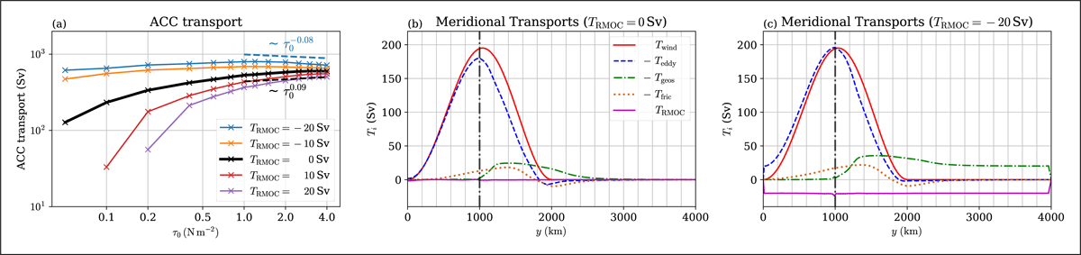
Figure 7
Diagnostics for GEOM, for a case where the wind is partially over the re-entrant channel (W02). (a) Diagnosed transport for different values of and . (b, c) Momentum balances for a zero and negative case, respectively; details are as in Figure 4. The vertical dashed-dot grey line denotes the model Drake passage separating the channel region and the basin region. The data scalings shown as black dashed line and blue dashed line are diagnosed via a regression over the indicated data range corresponding to the length of the dashed lines using data from the and calculation respectively.
Figure 7b,c shows the relative momentum balance for the zero and a negative case, respectively, for the same large wind forcing to describe the relative differences between the two cases. When is zero (panel b), the balance is between the Ekman and eddy components; however, in this case, the geostrophic component is non-negligible in the basin regions, as expected for the prescribed wind-forcing profile. When is negative (panel c), the effect of the imposed residual transport can be seen to be taken up by the geostrophic component away from regions of wind forcing, largely by the geostrophic and eddy components in the basin region with wind forcing (with a small friction contribution through the domain, except at the boundary regions), and by the eddy component in the channel region with wind forcing. The eddy terms are still significant over the channel region, and the eddy terms still exert a significant influence on the resulting transport and its sensitivity to wind forcing.
5.2 W23: wind solely over the basin
In the W23 case, the wind is solely over the basin region, so here we might expect the eddy component to play even less of a role compared to the previous cases. We show in Figure 8 the analogous diagnostics from the W23 calculation. Even though the wind forcing is not over the channel, a circumpolar transport is still possible (see, e.g., the analogous results in Marshall et al. 2016). An increase in the wind forcing over the basin region drives a larger western boundary current, and the non-trivial connection via the eddy component acting as a diffusion of h also leads to an increase in the circumpolar transport in the channel region. We see from Figure 8a that the circumpolar transport increases with increasing wind forcing for all cases, although the rate of increase is smaller when is negative. We show in Figure 8b,c the relative momentum balance for the zero and a negative case, respectively, for the same large wind forcing, to describe the relative differences between the two cases. When is zero (panel b), the geostrophic component is non-negligible, and it is of interest here that the eddy component can be locally of the opposite sign to the geostrophic component. When is negative (panel c), we observe that the presence of the residual component is reflected in a significant increase in the geostrophic component throughout the majority of the domain, leading to a notable decrease in the eddy component (except in the channel region where some of the residual leads to a non-zero eddy component). For this particular case, the geostrophic component is comparable to the eddy component, and when the wind forcing is increasing over the basin regions, the geostrophic component becomes increasingly present, and there is no strong constraint that the eddy component plays a dominant role. Under these conditions, although the open channel exists and there is a flow through it, the dynamics seen here are primarily gyre dynamics. However, this is not a Stommel gyre from the classic depth integrated theory, since the reduced-gravity system is baroclinic, which allows for a non-negligible eddy component. Channel dynamics have very little effect on the overall system.
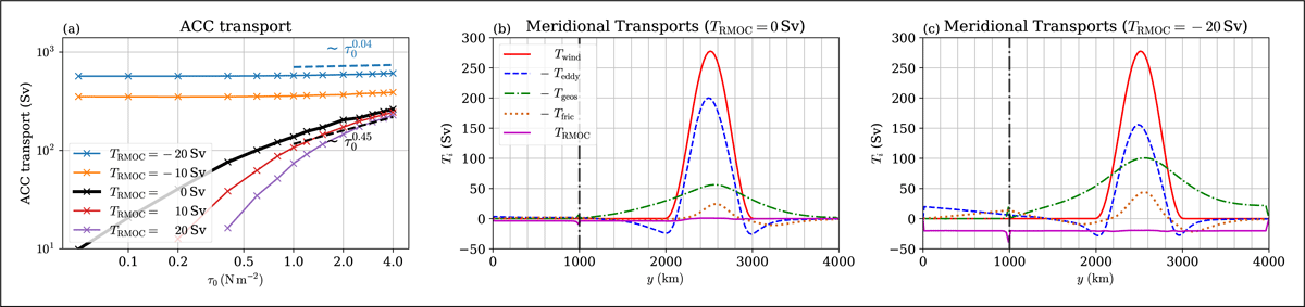
Figure 8
Diagnostics for GEOM, for a case where the wind is completely over the basin (W23). (a) Diagnosed transport for different values of and . (b, c) Momentum balances for a zero and negative case, respectively, for ; details are as in Figure 4. The vertical dashed-dot grey line denotes the model Drake passage separating the channel region and the basin region. The data scalings shown as black dashed line and blue dashed line are diagnosed via a regression over the indicated data range corresponding to the length of the dashed lines using data from the and calculations, respectively.
For completeness, the circumpolar transport for ML and CONST significantly increase with increases with wind forcing regardless of the choice of (cf. Figure 3) for both the W02 and W23 cases, since the eddy component in those two cases are even less dominant compared to the analogous GEOM calculations.
6 Conclusion
The sensitivity of modelled circumpolar transport to changes in forcing is of interest because the circumpolar transport is a key ocean climate metric, since the associated circumpolar transport is closely related to the global stratification to the north of the Atlantic Circumpolar Current (e.g., Fox-Kemper et al., 2019; Mak et al., 2022a; Munday, Johnson and Marshall, 2013). Several previous works have found that sometimes ocean models can have the curious behaviour that increasing wind forcing could lead to decreases in the modelled circumpolar transport, in quasi-geostrophic but eddying models (Youngs, Flierl and Ferrari, 2019), as well as primitive equation models that are eddy-rich or with parameterised eddies (Mak et al., 2018, 2023) if the residual overturning is in the negative sense. We term this phenomenon negative sensitivity in this work. Questions then arise as to the role of the eddies and the negative RMOC (interpreted in this model as a poleward above-pycnocline mass flux into the domain) in this negative sensitivity phenomenon.
In the present work, we specifically focus on the case where eddies refer to transient eddies, modelled as an eddy-induced advection with coefficient (e.g., Gent and McWilliams, 1990; Gent et al., 1995). Our model is based on Marshall et al. (2016), but differs in its choice of eddy parameterisations of form stress, imposed residual overturning circulation and the numerical implementation. Our analysis and results in Sec. 4 suggest that, in the present case, the GEOMETRIC parameterisation (Marshall et al., 2012; Mak et al., 2018, 2022a) together with the presence of a negative RMOC leads to a negative sensitivity (Figure 3a) via a sharpening of the baroclinic jet (Figure 5a). The sharpening occurs through the following physical mechanism:
A negative RMOC leads to a mass flux into the domain and contributes to the circumpolar transport, and in this case leads to a broadening of the channel jet and non-trivial contributions in the basin.
Increased wind forcing over the channel drives an increased eddy contribution via increases in the value of , which in turn diminishes the contribution from the negative RMOC.
The contribution from the negative RMOC is reduced, resulting in a reduction in the initial broadening, i.e., the jet sharpens.
This sharpening feature and decreased contribution from the negative RMOC is expected to be present in general, but only manifest as a negative sensitivity in GEOM. This is because GEOM allows for eddy saturation: the maximum jet profile magnitude is fixed and the wind contribution is independent of wind stress, but the negative RMOC contribution is damped, leading to a sharpening and decrease in total circumpolar transport. Negative sensitivity is not visible in ML and CONST simply because whatever reduction in the transport from the negative RMOC contribution is overwhelmed by the wind-driven contribution with increasing wind stress. As a consistency check, an optimisation calculation based on a linear decomposition of a wind stress-driven and RMOC-driven component was performed (cf. gyre and channel mode of Nadeau and Ferrari 2015, but we make no claims here that such a procedure here is anything but a zeroth-order consistency check). The calculation demonstrates consistency with the aforementioned mechanism. More work is, however, required to turn the present work into a quantitative predictive theory (e.g., investigating the actual structure of presumably western boundary flow driven by the negative RMOC, the nonlinear interactions), but our investigation in that direction is thus far inconclusive.
When the dominant balance is not between eddy and wind components, such as when there are non-negligible contributions to the overall momentum balance from the geostrophic and/or friction component (e.g., when the wind forcing is not solely over the channel), the analysis presented does not strictly hold. Nevertheless, the use of GEOM does generally lead to a reduction of the sensitivity of modelled circumpolar transport to changes in the wind forcing, in line with the stronger scaling of the eddy-induced velocity coefficient .
In the present work, a choice was made to perform the investigation in an idealised and simplified model, to isolate and highlight the plausible contributions of different processes. In other models with flow–topography interactions, standing eddies can result and have a significant contribution to the momentum balance (e.g., Mak et al., 2018, 2023; Masich, Mazloff and Chereskin, 2015; Stewart, Neumann and Solodoch, 2022; Youngs et al., 2017; Youngs, Flierl and Ferrari, 2019). We should note, however, that standing eddy fluxes across latitude circles are equivalent to transient eddy fluxes across time-mean streamlines (e.g., Marshall et al., 1993), and one needs to be a bit careful in attributing causality to the observed solution behaviour. From either point of view, we argue that standing eddies play a similar role to transient eddies in the sense that they both lead to form stress and counteract the increase in transport from the wind forcing. Eddy saturation and negative sensitivity could occur if the eddy effects have a strong enough scaling with the wind forcing, individually or in combination with each other, although the quantitative details will presumably differ. We speculate that inclusion of flow–topography interaction would alter the location in parameter space where eddy saturation and/or negative sensitivity occurs, possibly providing an explanation why we find negative sensitivity for rather large wind forcings here, when other works such as Youngs, Flierl and Ferrari (2019) and Mak et al. (2018; 2023) find these regimes in more realistic choices of wind forcings. An investigation in an analogous 2-layer model to the 1.5-layer model used here is possible to investigate the interplay between topographic steering effects and transient eddy contributions; however, this is beyond the scope of the present work.
One could argue that the negative sensitivity phenomenon occurs in a rather special limit where there is a poleward above-pycnocline meridional flow that is counter to the sense that is observed in the present climate, and is additionally only seen to occur when the GM-based GEOMETRIC parameterisation is active. This is certainly a valid point; however, we note that a similar phenomenon is also present in models with an explicit representation of mesoscale eddies, as we all as in cases where the RMOC is opposite to that of the present climate (e.g., Mak et al., 2018, 2023; Youngs, Flierl and Ferrari, 2019). While some of these may be due to the presence of the standing eddies, the present observation seems to suggest that the GM-based GEOMETRIC parameterisation is able to represent the related eddy–mean interactions even in this non-conventional limit, when other GM variants do not (and cannot, by our arguments in Sec. 4). Although we cannot claim that the GM-based GEOMETRIC scaling is the ‘correct’ one, the result does add to the growing evidence that the GM-based GEOMETRIC parameterisation can reproduce desirable aspects of eddy-rich models but in coarse resolution models (e.g., Mak et al., 2018, 2022a, 2023; Wei, Wang and Mak, 2024). The present work thus serves a secondary purpose in exploring sensitivities of model behaviour associated with the GM-based GEOMETRIC parameterisation in different ocean-relevant physical regimes. In addition, this result has interesting implications when considering palaeoclimates, as it is theorised that there were periods during which there was little to no North Atlantic Deep Water formation (Rahmstorf, 2002), and most of the deep water formation was focused on the Southern Ocean, possibly resulting in a reversal of the surface flow opposite to that of the current era (e.g., Zhang et al., 2022). If the surface flow had truly gone in the opposite direction, our theory suggests that negative sensitivity could have been present in those time periods.
Our model makes it possible in principle for us to look at different combinations of basin gyre and channel circumpolar flow, similar to the ‘gyre mode’ and ‘circumpolar mode’ theory proposed by Nadeau and Ferrari (2015). However, a direct comparison of our work with that theory is problematic, as their theory makes a linearity assumption where the forcing projects onto separate modes when the underlying system is nonlinear, and that work does not provide quantitative proposals for how one defines the gyre and circumpolar mode. While a comparison by eye is not entirely satisfactory, our general results (not shown) do not support Nadeau and Ferrari (2015)’s hypothesis that eddy saturation can be explained by strengthening gyres, but instead show the gyres strengthening with increasing wind stress regardless of whether eddy saturation is observed.
In the present work, we only focus on equilibrium responses, and the numerical method is chosen to take advantage of this, solving for the steady-state problem directly. The numerical solve time with the present methodology is on the order of minutes, compared with hours for pseudo-timestepping methods, and even days when the eddy energy budget is included, for a similar number of degrees of freedom and the same computational resources. The methodology allowed for a comprehensive scan throughout the parameter space, although we only report on a small but representative subspace in the present work. The numerical methodology and the use of the automatic code-generation software FEniCS (e.g., Alnæs et al., 2015) presented here (and the related software Firedrake, e.g., Rathgeber et al. 2017) is perhaps less well-known in the field of physical oceanography, but should be applicable in other idealised problems where the equilibrium response is the subject of focus (e.g., Allison et al., 2010; Howard et al., 2015; Huber and Nof, 2006; Johnson et al., 2007; Jones and Cessi, 2016; Munday et al., 2024).
The route towards equilibrium, i.e., the associated spin-up and adjustment problem (e.g., Allison, Johnson and Marshall, 2011) is also of interest from a theoretical point for understanding, and of numerical and observational point of view to inform on the length of numerical integration or data time series. The theoretical analysis pursued in this work assumes equilibrium balances, but there are feedback loops that are presumably inaccessible under the present methodology. In addition, the fact that GEOMETRIC utilises a parameterised eddy energy budget implies time-scales associated with the growth of eddy energy, coupled to the adjustments inherent in the mean-state, suggesting an oscillator-type behaviour. The work of Maddison et al. (2025) derives a nonlinear oscillator model motivated by that of Ambaum and Novak (2014) (see also Sinha and Abernathey 2016; Kobras et al. 2021; Ong et al. 2024) and makes a prediction of decay and oscillation time-scales associated with the mean and eddy adjustment. The associated investigation on adjustment time-scales and dynamical feedback loops is beyond the scope of the present investigation, but is currently being investigated and will be reported in subsequent publications.
Data Accessibility Statement
The numerical model code, analysis code and sample model data are available on Zenodo at http://dx.doi.org/10.5281/zenodo.15304142.
Appendices
Appendix A: Further Details on the Optimisation Calculation
The optimisation calculation encapsulated in the text around Eq. (31) relies on two non-dimensionalised basis patterns, so that the dimensional control variables a and b (the coefficients of the associated basis patterns) provide a measure of the respective magnitudes. The assumption relies on an approximate invariance of the chosen profile with changes in the wind stress (with a zero ), which is largely supported by the profiles shown in Figure A.1 (there is a meridional shift of the pattern in CONST with increased ). For the results presented in this work, we choose to take the pattern diagnosed from , normalised by the maximum value after a zonal average.
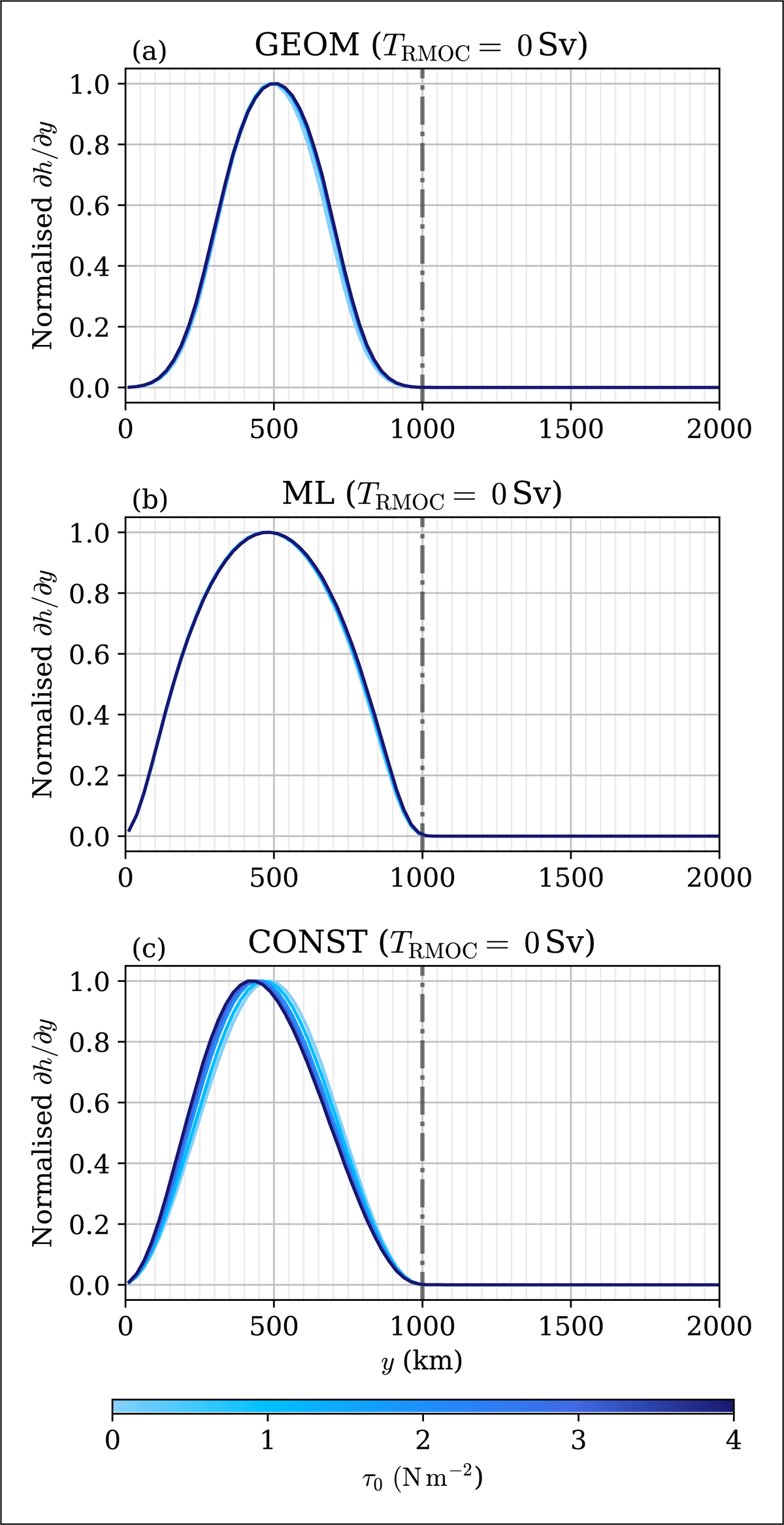
Figure A.1
The zonally averaged profiles of the W01 case (wind forcing only over the channel) at zero , normalised by the maximum of the zonally averaged profile. (a) GEOM, (b) ML and (c) CONST. The vertical dashed-dot grey line denotes the model Drake passage separating the channel region and the basin region.
The optimisation procedure was implemented in Python using scipy.optimize.minimize with the default settings. The presented results use the squared L2 norm (i.e., ); other choices of norm were considered but not presented. The results presented here use the zonally averaged profile. The use of the zonally averaged u would give similar results, although computing the implied transport becomes more complicated since a thickness factor h is missing. The use of the zonally averaged h has the added complication that the normalised profiles were not as universal as the zonally averaged u or profiles (not shown). We have not attempted an optimisation calculation with a two-dimensional basis pattern, although that is in principle possible (using just scipy.optimize.minimize, doing a linear solve of a 2 by 2 matrix, or leveraging FEniCS capabilities). The qualitative conclusions drawn from Figure 6 were found to be robust from the different combinations of basis variables, norms and optimisation routine parameters considered (not shown).
A sample of the profile from the optimisation calculation and the target profile is shown in Figure A.2. The deviations arise from the incomplete nature of the linear decomposition, which is not entirely surprising given that the equations are nonlinear. The optimisation procedure is unable to represent the secondary jet formed over the basin in GEOM and ML, but does capture the bulk aspects of the diagnosed profiles. The present approach provides a qualitative check on the consistency of the proposed physical mechanism, but more work is required for this to be a quantitative theory.
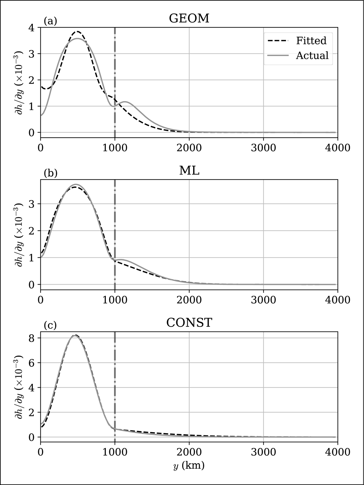
Figure A.2
The profile returned by the optimisation calculation (black dashed) and the actual diagnosed profile (grey), for the case ad , for (a) GEOM, (b) ML and (c) CONST.
Acknowledgements
We extend our thanks to Jonas Nycander and the two other anonymous referees for their many valid comments, which made us think about the problem more thoroughly, leading to an improvement in the scientific content and presentation of the article (Jonas Nycander is particularly acknowledged for some material that is now included in Sec. 4.1 and 4.2).
Competing Interests
The authors have no competing interests to declare.
Author Contributions
Resources, Supervision, Project administration, Funding acquisition: JM. Conceptualization, Visualization, Methodology: HSL, JM, DPM, JRM. Software, Formal Analysis, Validation: HSL, JM. Writing – Original Draft: HSL, JM, DPM, YW. Writing – Review & Editing: everyone.
Author Note
For the purposes of open access, the authors have applied a Creative Commons Attribution (CC-BY) license to any Author Accepted Manuscript version arising from this submission.