
1 Introduction
The major weakness of Observing System Simulation Experiments (OSSEs) is the reliance on a completely simulated framework, raising questions about the relevance of the experimental results to numerical weather prediction (NWP) in the real world. There are multiple aspects of the OSSE framework that only imperfectly reproduce the real world and therefore may not properly characterize the impacts of potential new observing systems. This can be partially mitigated in practice by careful validation of the OSSE (Arnold and Dey, 1986; Atlas, 1997; Halliwell et al., 2014; Hoffman and Atlas, 2016; Boukabara et al., 2018; Errico and Privé, 2018; Yu et al., 2019) against real world NWP, but some aspects of the OSSE are difficult to validate because the characteristics of the real world system are not adequately known.
An NWP OSSE framework consists of several components. The real atmosphere is represented by a Nature Run (NR), typically a long, free run of a high resolution NWP model. The NR replaces the real world both for the purposes of generating simulated observations, and for verification of the experiment results. An advantage of the use of a NR is that the entire true state of the NR is known, unlike the real atmosphere, allowing direct calculation of quantities such as the analysis and background errors. Simulated, or synthetic, observations are generated by spatiotemporal interpolation of the NR fields along with the use of observation operators for data types such as radiances or radio occultation. All data types that are used operationally in NWP should be simulated to fully recreate the global observing network in the OSSE. Observation errors are simulated and added to the synthetic observations to account for representativeness, operator, and observation errors that may be deficient otherwise. The simulated observations are then ingested into a second NWP model and data assimilation system (DAS) using methodology identical to that used for real observations. The OSSE framework allows the simulation and testing of many different observation configurations, and may be used not just for investigations of proposed new observing systems but also for evaluation of the performance of the DAS in a highly controlled but sophisticated environment.
One aspect of OSSEs that can strongly affect the overall behavior of the entire system is insufficient model error, or ‘twinning’. In general, OSSEs tend to have less model error compared to real world models because any two NWP models are more similar to each other than either model is to the real world. Thus, when one NWP model is used to generate a NR, any model that is chosen for running NWP experiments will tend to have better forecast skill in correspondence to that Nature Run than the same model would have in correspondence to the real world (Privé et al., 2013b; Yu et al., 2019). The apparent model error in the OSSE can be increased somewhat by using two models respectively for the Nature Run and experiment forecasts that have as different as possible resolutions, physics parameterizations and schemes, and dynamical cores (Halliwell et al., 2014; Hoffman and Atlas, 2016) with the constraint that both models are sufficiently realistic. However it is also sometimes necessary to perform a so-called ‘twin’ OSSE in which a similar (‘fraternal twin’) or the same (‘identical twin’) model is used for both the Nature Run and for the experiment forecasts.
Yu et al. (2019) compared the impact of ocean observations in an identical twin OSSE setting to a fraternal twin setting and found that the identical twin configuration lead to overestimates of the impact of some observations and underestimates of other observation impacts. They also found that achieving a realistic model error growth rate was not sufficient to yield accurate observation impacts in an OSSE. Privé and Errico (2013b) compared the simulated error growth rates in identical twin and fraternal twin OSSE versions and found that while the forecast errors were considerably lower in the identical twin OSSE, the error growth rates were somewhat similar between the fraternal and identical twin OSSEs. It is therefore of interest to evaluate how twinning in the atmospheric OSSE framework affects the results of experiments evaluating the impacts of proposed new instruments in atmospheric OSSEs.
Another frequent deficiency of OSSEs is the use of an outdated forecast model and DAS, along with a simulated global observing network that may be based on the real world observations several years previous. For example, the 1990s-era OSSE framework developed by Bloom et al. (1996) was used for more than a decade (Cardinali et al., 1998; Stoffelen et al., 2006; Masutani et al., 2010), and the Nature Run produced by the National Aeronautics and Space Administration Global Modeling and Assimilation Office (NASA/GMAO) in 2014 is still in use today. OSSEs require a substantial investment in computing resources and development, and as such tend to lag behind the current operational NWP systems. While OSSEs are periodically updated to reflect advances in the operational system, it is not possible to keep completely abreast with the real world. Given that OSSEs are most often used to evaluate the potential performance of future proposed instruments, there is a question of how well the OSSE experiment results represent impacts in a future NWP system when the global observing system and data assimilation systems may differ substantially from the current systems.
The GMAO global OSSE framework (Errico et al. (2017)) has recently been updated, affording an opportunity to explore some of these questions. This framework uses a Nature Run produced at high spatial and temporal resolution by an earlier version of the Goddard Earth Observing System (GEOS) model. A more recent version of GEOS at lower horizontal resolution is employed for the NWP experiment model in the OSSE, so the GMAO OSSE framework can be considered a fraternal twin OSSE. The transition from the ‘Previous’ to the ‘Updated’ version of the GMAO OSSE included changes both to the simulated global observing network and to the DAS as well as the physics and dynamics of the NWP model used for the experiments. The global observing network was based on the data types used operationally in 2015 for the Previous OSSE framework, and on the 2020 global observing network for the Updated framework. The version of GEOS used for the NWP experiments in the Previous OSSE had relatively similar atmospheric physics and dynamics to the Nature Run model, while numerous changes to the convection, radiation, and boundary layer schemes, as well as to the dynamical core were made to GEOS in the Updated framework. The Updated OSSE framework is therefore expected to be less of a twin OSSE than the Previous OSSE framework.
First, the performance of the Updated OSSE framework will be validated compared with the real world NWP behavior. This is important in order to fully place the OSSE experiment results into context with the real world. The Updated framework includes new data types, including all-sky treatment of the Microwave Humidity Sounder (MHS), Advanced Microwave Scanning Radiometer 2 (AMSR2), and Global Precipitation Measurement (GPM) Microwave Imager (GMI) observations. The Updated OSSE framework has also been extended a third month into September beyond the July-August timeframe of the Previous OSSE. The degree of twinning in the Updated OSSE framework will be explored and compared with the Previous OSSE framework. The effects of insufficient model error on several different aspects of OSSE performance will be characterized, including simulated observation error calibration, analysis increments, background error, forecast skill, and observation impacts.
Several new observing types were tested in both the Previous and Updated OSSE frameworks. These instruments are the Geostationary eXtended Observations (GeoXO) hyperspectral infrared sounder (GXS) (McGrath-Spangler et al., 2022), additional Global Navigation Satellite System Radio Occultation (GNSS-RO) observations (Privé et al., 2022), and atmospheric motion vectors for the Midwave Infrared Sounding of Temperature and humidity in a Constellation for Winds (MISTiC Winds) instrument (McCarty et al., 2021). Select experiments for each of these instruments were repeated in both OSSE frameworks to compare how the observation impacts of the new instruments are affected by the framework used. The observation impacts on metrics such as analysis quality, forecast skill, and Forecast Sensitivity Observation Impact (FSOI) will be compared in the two OSSE frameworks for each instrument in connection to changes to the background error, model error growth, and global observing network.
This manuscript is organized as follows: the OSSE framework is described in Section 2 and validated, including evaluation of the model error in the Previous and Updated OSSE frameworks, in Section 3. The observation impacts from three different proposed instrument types are compared between the Previous and Updated OSSE frameworks in Section 4. The results of these evaluations will be discussed in Section 5.
2 OSSE Framework
The GMAO global NWP OSSE framework has been updated to a recent (circa 2022–2023) quasi-operational version of the GEOS model and Gridpoint Statistical Interpolation (GSI) data assimilation system, with simulated observations based on the 2020 global observing network. The Previous version of the GMAO OSSE framework used the GEOS/GSI versions that were in use quasi-operationally in 2018, with simulated observations based on the global observing network in 2015. That version has been extensively documented (Errico et al., 2013; 2017; Privé et al., 2021; 2022; El Akkraoui et al., 2023), and multiple OSSE studies have been performed using that framework (Privé et al., 2022; McGrath-Spangler et al., 2022; Privé et al., 2023). The following discussion will give a brief overview of the GMAO NWP OSSE framework, with focus on the changes implemented in the Updated version.
2.1 Nature Run
The Nature Run (NR) is a long, free model run that acts as the ‘truth’ in the OSSE in place of the real atmosphere, and is also used as the basis for generating simulated observations. Ideally, the Nature Run should have high spatiotemporal resolution and the most realistic parameterizations available. The Nature Run must be able to capture both the phenomena of interest for the experiments, and also all the fields necessary for simulation of the global observing network.
A two-year long forecast of the GEOS model at 7 km horizontal resolution with 72 vertical levels and 30-minute output is used as the Nature Run for both the Previous and Updated OSSE frameworks. This Nature Run is generally referred to as the “G5NR”. The version of GEOS used to generate the NR dates approximately to 2014 and is similar in nature to the model version used for MERRA-2 (Molod et al., 2015). The G5NR has been extensively validated as documented in Gelaro et al. (2014).
2.2 Forecast Model
The NWP model used for the experiments is the version of GEOS (Rienecker et al., 2008) that was quasi-operational in 2022–2023, run with 25 km horizontal resolution (C360) and 72 vertical levels, and will be referred to as the Updated framework. This model differs from the version of GEOS used for the Nature Run in terms of the resolution, the advection schemes for thermodynamic and momentum variables, higher order divergence damping schemes, the land model, the convective and radiation schemes, and the boundary layer parametrizations. The model used in the Previous version of the OSSE framework (El Akkraoui et al., 2023) was the GEOS version that was quasi-operational in 2018, and that had fewer differences from the NR model, with very similar radiation and boundary layer schemes. It is expected that the Updated model version will have better simulation of model error in the OSSE framework as a result of more substantial differences between the experiment model and the NR model versions.
The data assimilation system used in the Updated version is the hybrid 4-dimensional ensemble variational (4DEnVar) GSI. The major differences between this version of GSI and that used in the Previous OSSE framework are the all-sky treatment of GPM/GMI, MHS, and AMSR2 observations and an update to the incremental analysis update (IAU) scheme.
2.3 Synthetic Observations
Simulated observations are generated for existing real-world data types that were used quasi-operationally during a corresponding timeframe. For the Updated OSSE, this timeframe is summer 2020, while the Previous framework was based on the 2015 global observing network. A comparison of the data types used in the Previous and Updated systems is shown in Table 1. The goal of simulating observations is to represent what the observations would have been if the real atmosphere were replaced with the NR during that time period, including both the spatiotemporal distribution of the observations and the statistical quality of the data as used by the data assimilation system. Ideally, a randomly selected subset of the simulated observations would not be easily distinguished from real observations.
Table 1
Simulated observing platforms for the Previous (2015) and Updated (2020) GMAO NWP OSSE frameworks.
| INSTRUMENT | PLATFORM | 2015 | 2020 | ALL-SKY | CORRELATED ERRORS |
|---|---|---|---|---|---|
| AIRS | Aqua | X | X | Channel | |
| AMSR2 | GCOM W1 | X | 2020 | ||
| AMSU-A | Aqua | X | Horizontal | ||
| AMSU-A | NOAA-15 | X | X | Horizontal | |
| AMSU-A | NOAA-18 | X | X | Horizontal | |
| AMSU-A | NOAA-19 | X | X | Horizontal | |
| AMSU-A | METOP-A | X | X | Horizontal | |
| AMSU-A | METOP-B | X | X | Horizontal | |
| AMSU-A | METOP-C | X | Horizontal | ||
| ATMS | NOAA-20 | X | Horizontal | ||
| ATMS | NPP | X | X | Horizontal | |
| CrIS | NPP | X | Channel | ||
| CrIS-FSR | NPP | X | Channel | ||
| CrIS-FSR | NOAA-20 | X | Channel | ||
| GMI | GPM | X | 2020 | ||
| HIRS4 | METOP-A | X | Horizontal | ||
| IASI | METOP-A | X | X | Channel | |
| IASI | METOP-B | X | X | Channel | |
| MHS | NOAA-18 | X | Horizontal | ||
| MHS | METOP-A | X | Horizontal | ||
| MHS | METOP-B | X | X | 2020 | Horizontal |
| MHS | METOP-C | X | 2020 | Horizontal | |
| SSMIS | F17 | X | X | Horizontal | |
| Surface conventional | X | X | |||
| AMV | X | X | Horizontal, Vertical | ||
| Aircraft | X | X | |||
| Scatterometer | X | X | |||
| RAOB | X | X | Vertical | ||
| GNSS-RO | X | X | Vertical |
For many observing system types, the spatiotemporal location of observations can be based directly on the corresponding locations of real data. For example, surface observations, GNSS-RO, or satellite orbits may be based on the locations of real data. These observations may be simulated by interpolating the NR fields to the location of real observations, and possibly the additional use of an observation operator, e.g. a radiative transfer model, to convert the model fields to the variables measured by the instrument. A thorough description of the methodology used in the GMAO OSSE framework is given by Errico et al. (2017), with updates to the simulation of Atmospheric Motion Vectors (AMVs) discussed in Errico et al. (2020). GNSS-RO observations are simulated using the Radio Occultation Processing Package two dimensional operator (Culverwell et al., 2015). Rawinsondes and dropsondes are launched at the same time and location as real sonde releases, but are advected with the NR wind field. Aircraft observation locations, however, do not account for wind-routing of flight tracks.
Radiance observations are generated using the Community Radiative Transfer Model (CRTM; Han et al. (2006); Ding et al. (2011)) version 2.2.3 for both the Previous and Updated OSSE frameworks. While geolocation of radiance observations are taken from real observations, the NR cloud field is used to determine observation locations (Errico et al., 2013) for clear-sky radiances. The radiance types treated as all-sky observations (GMI, MHS, and AMSR2) used the NR fields of liquid, frozen, and vapor moisture and precipitation to produce cloud-affected radiances. An example of a simulated GMI channel compared with real GMI is shown in Figure 1, illustrating the close match of the distribution of observation innovations (O-B), with the simulated observations reflecting the locations of NR moisture fields. Several types of radiance observations suffered significant outages during 2020. For any radiance type that experienced an outage of more than one cycle time, the locations of 2021 observations for that data type on the same day of the year were substituted for simulation of that instrument.
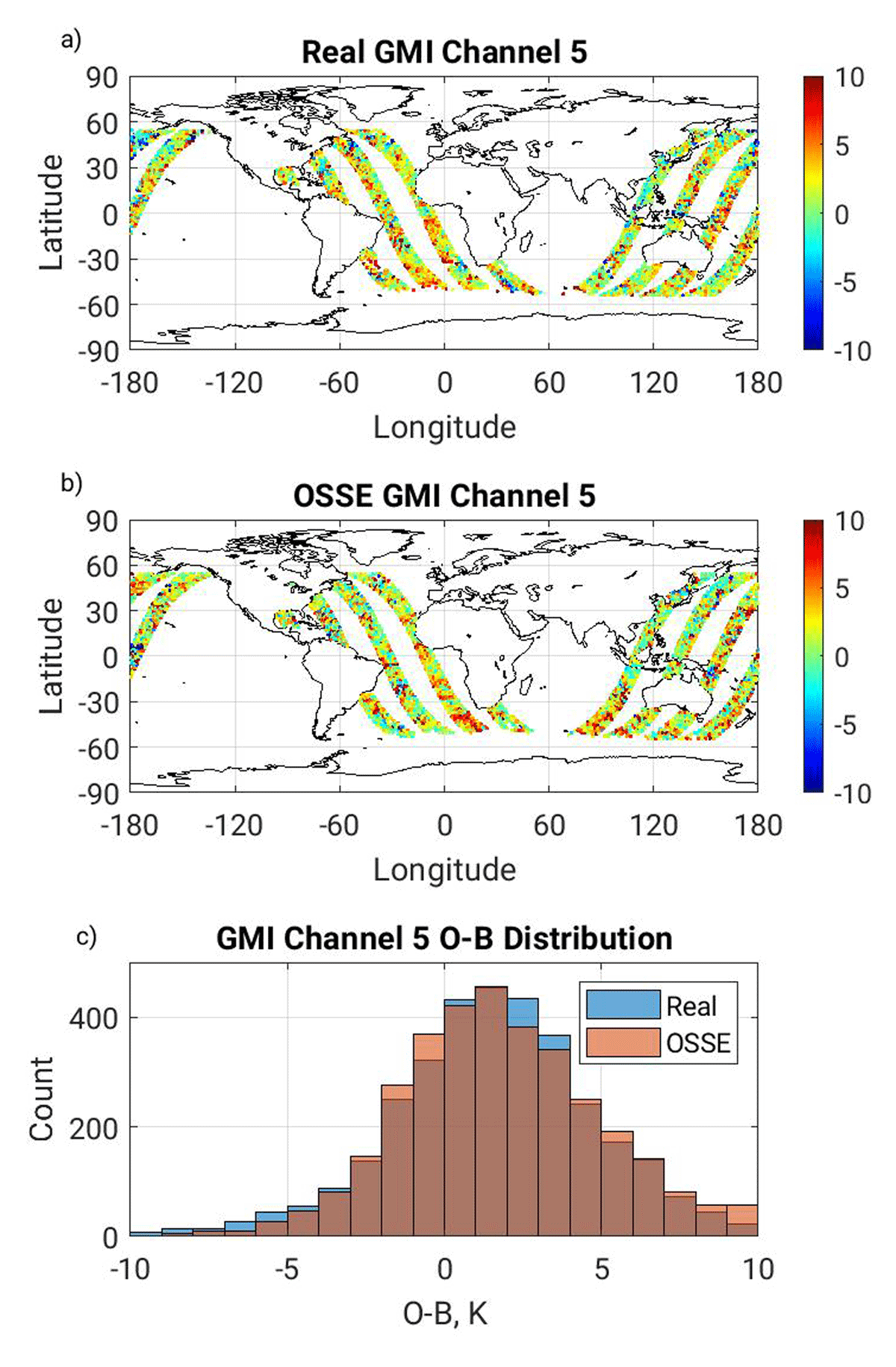
Figure 1
Comparison of real and simulated GMI observations for channel 5 on 10 July 00z in the Updated OSSE framework. a) Real GMI with brightness temperature O-B in color, K. b) Simulated GMI with brightness temperature O-B in color, K. c) histogram of brightness temperature O-B for Real and simulated GMI observations.
Similarly, AMVs are based on the location of cloud and water vapor features in the NR modulated by the footprint of the corresponding satellites (Errico et al., 2020). One exception to this is the simulation of Himawari AMVs in the 2020 dataset, where the distribution of simulated observations using the NR fields was not representative of the grid-like characteristics of real observations, so the corresponding real observation locations were used for simulation.
2.3.1 Calibration
Simulated observation errors are added to most simulated data types following the methodology described in Errico et al. (2013) and Errico et al. (2017). Uncorrelated random errors are added to all data types, and random correlated errors are added to select data types as noted in Table 1. The magnitude of the simulated errors and the characteristics of the error correlations are adjusted to match the statistics of real observations (Privé et al., 2021).
The calibration process involves adjusting the statistical thresholds used to determine cloud effects for the simulated observations to match the counts of real observations, and also tuning the simulated observation errors until the variance of the observation innovations matches that of real data. This process is performed for a weeklong period at the end of June prior to the start of the experiment timeframe on 1 July. The short period is rerun numerous times while making adjustments until the calibration is satisfactory. This period also allows for the spinup of the radiance bias correction, with the iterative process over the same short period adding up to several months of adjustment for the bias correction coefficients.
Figure 2 compares the standard deviation of observation innovations for several real and simulated radiance instruments for the month of July. The OSSE statistics for simulated observations are relatively close to real statistics for most channels. The tuning of the error coefficients and cloud probability functions is expected to be seasonally dependent. Figure 3 compares the calibration of IASI Metop-A observation innovations for July, August, and September. Some deviation of the simulated observations from real is noted in the September timeframe, but the difference is not sufficient to warrant recalibration. A short test of the October timeframe (not shown) indicates that the calibration does not hold well beyond the end of September, possibly due to seasonal changes in the climatology of the G5NR.
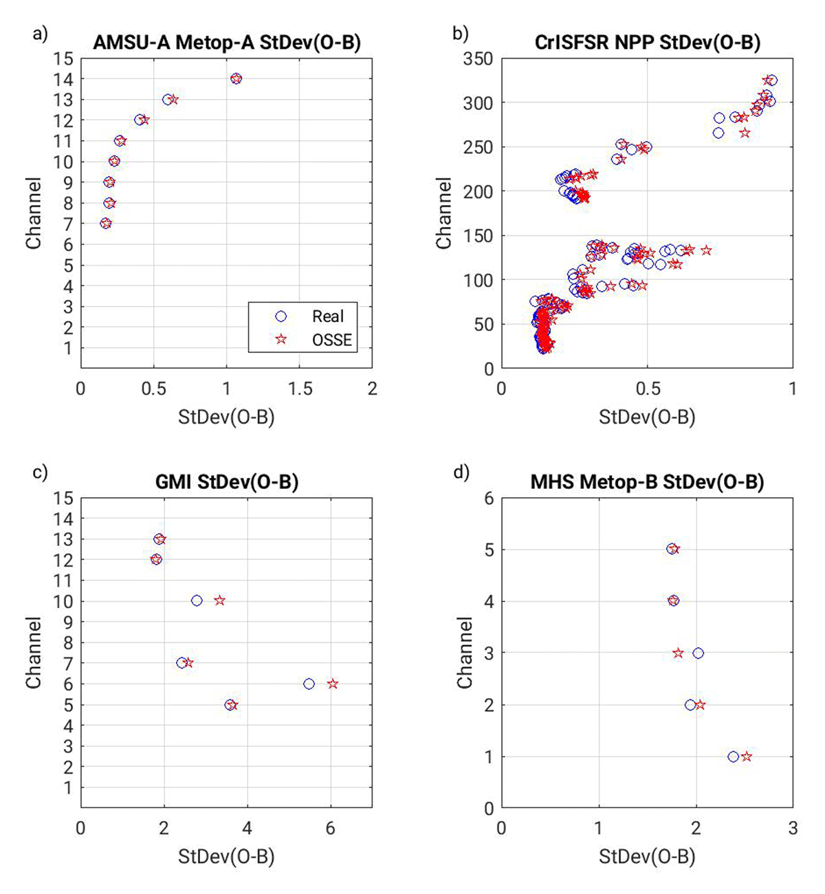
Figure 2
Comparison of standard deviation of real and simulated brightness temperature observation innovations for the month of July in the Updated OSSE framework. Blue circles, Real case; red starts, OSSE Control. a) AMSU-A Metop-A; b) CrIS NPP; c) GMI GPM; d) MHS Metop-B.
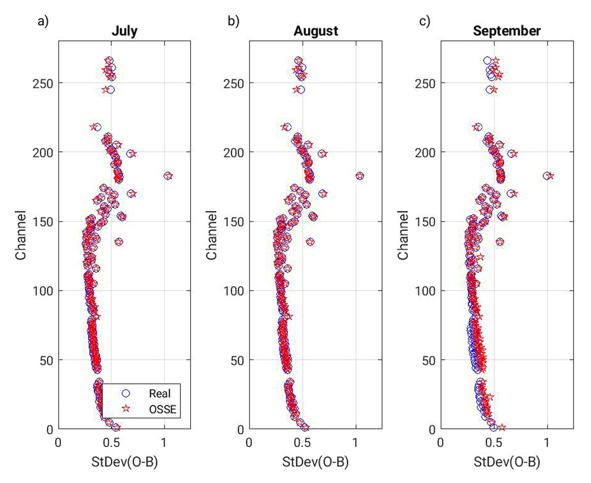
Figure 3
Comparison of standard deviation of real and simulated observation innovations for IASI Metop-A in the Updated OSSE framework. Blue circles, Real case; red starts, OSSE Control. a) July; b) August c) September.
2.4 OSSE Control
The OSSE Control run ingests only those data types available in the quasi-operational real system and acts as a basis of comparison for experiments in which new observing platforms are tested. The Control run is also used to validate the performance of the OSSE framework, employing a corresponding Real case with the same model and DAS versions run with real data for the time period used as a basis for the simulated observations (2015 for the Previous OSSE and 2020 for the Updated OSSE). The Updated framework Control run was expanded to the period of July-September in the second year of the G5NR. This is an extension of the Previous framework period of July–August. September was included in the Updated framework in order to capture the Atlantic basin tropical cyclone season in support of several proposed missions.
Initialization of the OSSE framework began at the start of June, with initial conditions taken from a pre-existing real world run. The GEOS/GSI was run in 3D variational mode for several days while ingesting a global network of highly idealized simulated rawinsonde-type observations arranged on a global grid in order to pull the model state closer to the NR state. The system was then switched to the standard set of simulated observations that mimic the real world global observing network, and the 32-member ensemble was spun up for a period of approximately three weeks.
After completing calibration of the simulated observations during the late June period, observations were produced for this entire time period. The OSSE Control was initialized from the end of the calibration period, and an ensemble run was performed for the entire period of interest. In addition to cycling the DAS, 10-day forecasts were produced daily initialized at 0000 UTC, along with FSOI also at the 0000 UTC cycle time.
The Previous OSSE framework Control was similarly executed for the period July–August, as described in detail in Privé et al. (2022) and El Akkraoui et al. (2023) and illustrated in Privé et al. (2020), Privé et al. (2021), and Privé et al. (2021).
3 OSSE Evaluation
Evaluation and validation of the OSSE framework encompasses multiple aspects of the NWP system, including the analysis increments, forecast skill, and observation impacts. These characteristics of the OSSE are not directly manipulated in the fashion of the observation characteristics, and are instead emergent qualities affected by both the simulated observations and the forecast error growth.
3.1 Background Error
The background error in the OSSE can be directly calculated using the NR fields as verification, but cannot be calculated for real systems because the true state of the atmosphere is not known. Figure 4 shows the zonal mean root-temporal-mean-square (RTMS) background error for temperature, humidity, and zonal wind for both the Previous and Updated OSSE Control cases. For temperature, there are localized maxima of RTMS error in the lower troposphere in the polar boundary layers and also associated with low cloud decks over cold maritime waters, such as off the west coast of South America. Humidity background errors are greatest in the tropical lower troposphere, where the specific humidities are much larger than in the colder latitudes or upper troposphere. The greatest zonal wind background error is associated with the upper level equatorial easterly jet, with local maxima near the two extratropical westerly jets at the tropopause.
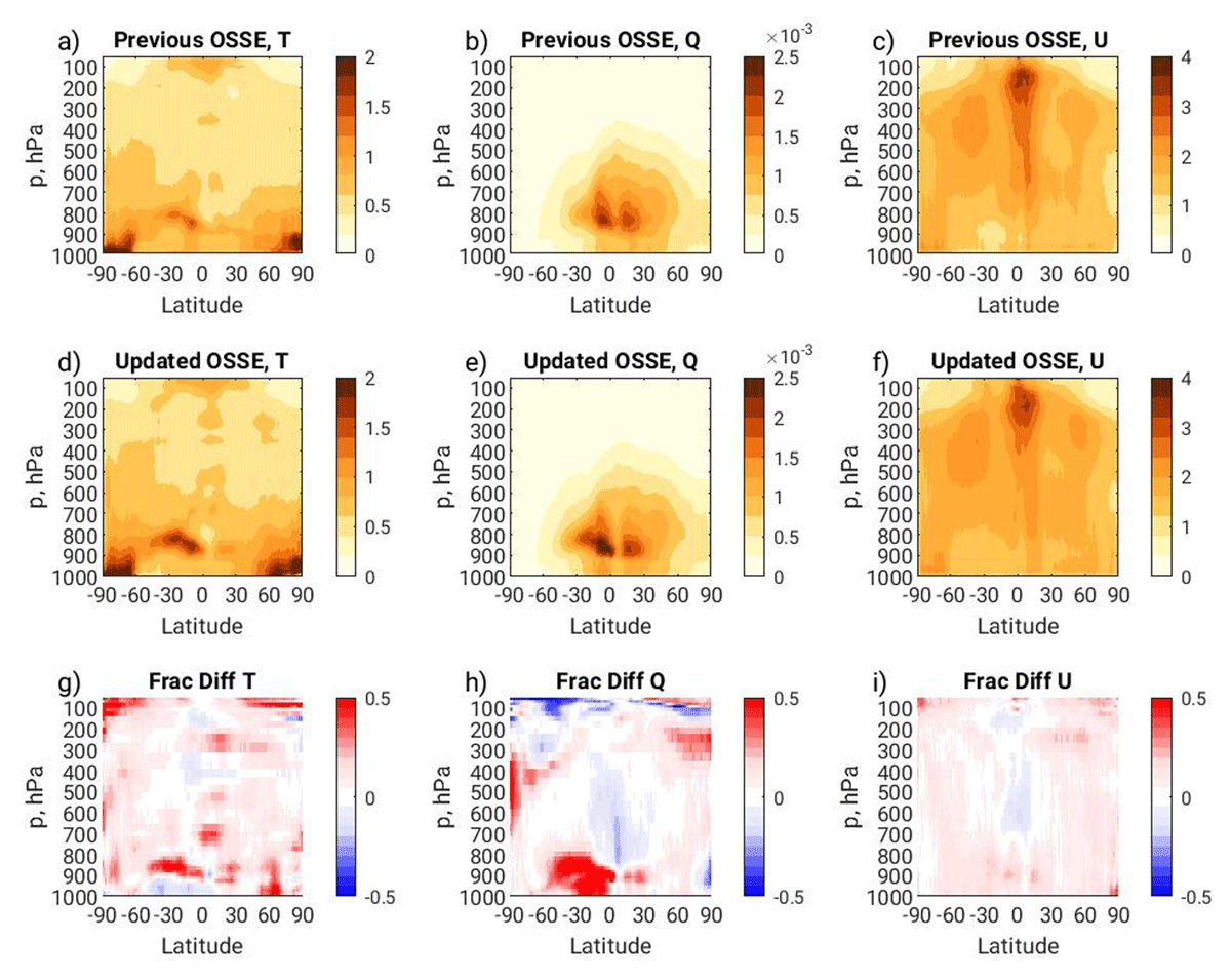
Figure 4
Zonal mean RTMS background error for the OSSE Control for the month of July, four times daily data. a,b,c) Previous OSSE framework; d,e,f) Updated OSSE framework; g,h,i) Fractional RTMS difference between frameworks, (Updated-Previous)/Previous. a,d,g) Temperature, K; b,e,h) specific humidity Q, kg kg–1; c,f,i) zonal wind, m s–1.
In the real world system, the newer DAS and model used in the Updated framework would be expected to have less background error than for the older DAS and model used in the Previous framework. However in the OSSE, the substantial changes to the GEOS model between the versions used for the Previous and Updated OSSE frameworks should introduce larger differences between the Updated OSSE and the NR compared to the Previous framework, which would tend to increase background error in the Updated OSSE. The overall change in background error in the OSSE framework depends on the relative contributions of these two opposing tendencies. As illustrated in the bottom row of Figure 4, the net tendency is for overall increases in background error in the Updated OSSE framework of 5–10%, with some localized variation.
The background error affects the calibration of the simulated observations in the OSSE. The magnitude of simulated observation error added to the simulated observations is adjusted during the calibration process to match the standard deviation of the observation innovations, O-B, to real observation innovations. If the standard deviation of the background error is smaller in the OSSE than in the real world, the simulated observation error in the OSSE may be overinflated compared to real observation errors in order to compensate. The relationship between the standard deviation of O-B and the variance of the background field is shown in the following equations:
It is assumed that the background error and observation errors are independent so that the covariance, cov(O,B) = 0. Thus it is expected that if the variance of background error in the OSSE framework, var(B), increases, then the magnitude of the variance of simulated observation error, var(O) needed to match real observation innovation standard deviations, stdev(O – B), will decrease. Figure 5 compares the magnitude of the standard deviation of simulated observation error added to the simulated rawinsonde observations in the Previous and Updated OSSE frameworks. Through most of the troposphere, the simulated rawinsonde errors in the OSSE have smaller magnitude in the Updated OSSE framework. Notably for temperature, there is a particularly large drop in the simulated rawinsonde errors in the Updated framework at 900 hPa, corresponding to a level where an especially large increase in background error is noted in Figure 4g.
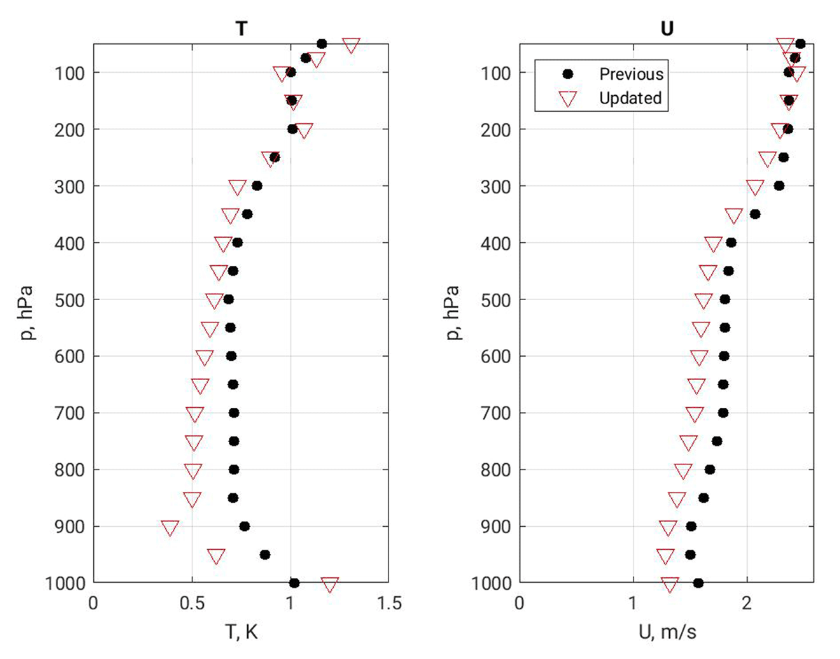
Figure 5
Magnitude of standard deviation of simulated observation error added to simulated rawinsondes in the Previous (black circles) and Updated (red triangles) OSSE frameworks. a) Temperature, K; b) Zonal wind, m s–1.
3.2 Analysis Increments
The zonal mean standard deviations of analysis increments (A-B) for the July–September period are illustrated in Figure 6 for temperature, humidity, and zonal wind for the Updated OSSE framework and corresponding Real data case. The analysis increments for the Updated system can be compared with a similar figure in Privé et al. (2021) for the Previous OSSE framework. In general, it has been found that OSSEs tend to have smaller magnitudes of analysis increments compared to real systems. This can be affected in part by the observations (Privé et al., 2021) but is also a reflection of the model error growth between cycle times. It is clear from the bottom row in Figure 6 that the analysis increments in the OSSE are weaker than for the real world, although the spatial structure of the increments is well represented in the OSSE. The magnitude of standard deviation of analysis increments in the OSSE is generally within 20% of the magnitude of real world increments in the Updated framework, compared to analysis increments that were 30% weaker than the Real case in the Previous OSSE framework.
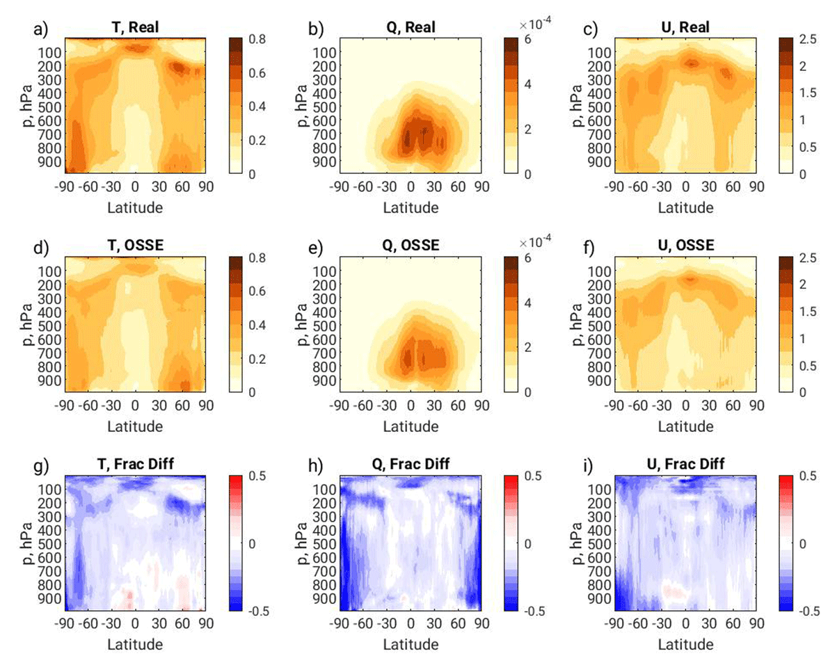
Figure 6
Standard deviation of analysis increment (A-B) for the month of July, four times daily data, for the Updated OSSE framework. a,b,c) Real; d,e,f) OSSE; g,h,i) Fractional difference of standard deviation of analysis increments, (OSSE-Real)/Real. a,d,g) Temperature, K; b,e,h) specific humidity Q, kg kg–1; c,f,i) zonal wind, m s–1.
3.3 Forecast Skill
The regional root-areal-mean-square errors (RAMS) for the 5-day forecast period in the Updated OSSE framework averaged over the three-month period are compared with real world forecast errors in Figure 7 by normalizing the OSSE forecast error statistics by the Real forecast error statistics. For consistency, the RAMS forecast error statistics for the OSSE Control and Real cases are calculated using self-analysis for verification for each case. Note that the analysis state generated by applying an analysis increment to the background field is used throughout this manuscript as the ‘analysis’, differing from the actual model state that is produced by integration of the forward model using the Incremental Analysis Update procedure implemented at GMAO (El Akkraoui et al., 2023). Correlations between short term forecast errors and self-analysis errors can result in substantial underestimations of short-term forecast errors for both Real and OSSE. The fractional forecast error statistics are not expected to approach 1.0 with extended forecast period even as forecast errors saturate due to the use of self-analysis verification, with different analysis states used for the OSSE and Real cases respectively. If the bias and/or variance of the analysis errors are weaker in the OSSE compared to real, the RAMS error-saturated forecast skill will have smaller magnitude and the fractional error will be less than one. The Previous OSSE (heavy black lines) is compared with the Updated OSSE (thin red lines).
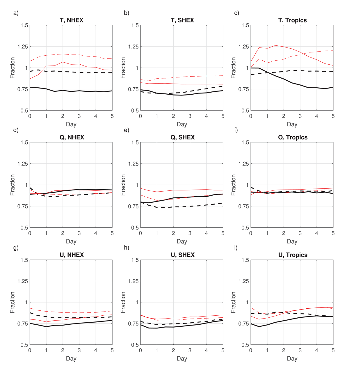
Figure 7
Comparison of root-areal-mean-square forecast errors for the OSSE Control vs Real, using self-analysis verification. Lines indicate the RMS OSSE Control forecast error normalized by the Real forecast error statistics for the month of July. The dashed lines are for 857 hPa, and the solid lines are for 266 hPa. Heavy black lines indicate the Previous OSSE, thin red lines indicate the Updated OSSE. (a)–(c) Temperature, K (d)–(f) specific humidity, kg kg–1, and (g)–(i) zonal wind, m s–1. (a),(d),(g) 20N–90N; (b),(e),(h) 20S–90S; and (c),(f),(i) 20S–20N.
OSSE temperature forecast RAMS errors in the troposphere are within 25% of the real case forecast RAMS errors, with equal or higher fractional error in the Updated OSSE framework compared to the Previous framework. For some levels and regions, the OSSE temperature forecast RAMS errors in the Updated system are greater than in the real system, such as for tropical temperatures, which may be related to changes in the model convective scheme. Humidity forecast RAMS errors and zonal wind forecast RAMS errors are somewhat smaller in the OSSE than in the real system, with relatively consistent deficiencies in RAMS error over the five day forecast period, and RAMS errors that are closer to the real system in the Updated OSSE compared to the Previous OSSE.
Figure 8 compares the RAMS forecast error for temperature, humidity, and zonal wind calculated with NR verification in the Previous and Updated OSSE Controls. Temperature at 500 hPa shows significantly greater RAMS forecast error in the Updated framework in the Tropics and Northern Hemisphere extratropics, but little difference in the Southern Hemisphere extratropics. This may be due to seasonal differences, with model-differing convective processes being more dominant in the tropics and summer hemisphere, and baroclinic processes dominant in the winter hemisphere. A diurnal cycle in forecast error is noted in the Updated framework most strongly in the Tropics but also to a slight degree in the Northern Hemisphere extratropics, likely due to the use of only forecasts for the 0000 UTC cycle time. Specific humidity in the lower troposphere demonstrates significantly greater forecast error in the Updated framework in all regions. The humidity RAMS errors are greater not only at the initial time, but there is an increased separation of the error curves as the forecast progresses, indicating faster error growth in the Updated framework compared to the Previous framework.
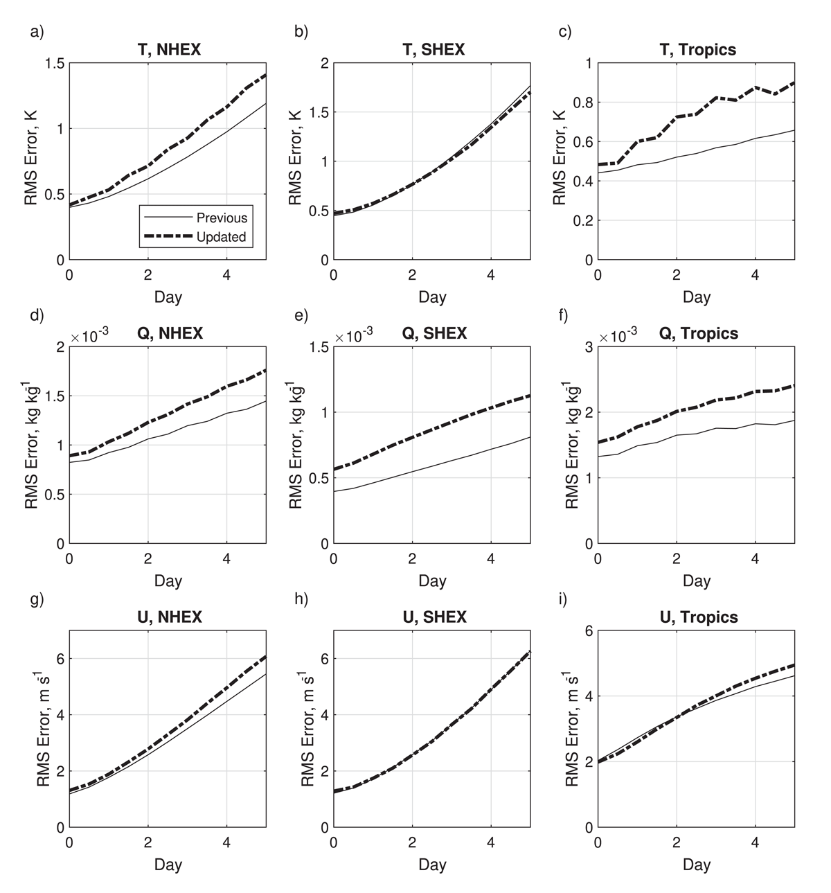
Figure 8
Comparison of root-areal-mean-square forecast errors for the OSSE Control in the Previous and Updated frameworks, using NR verification. The thin solid line is for the Previous OSSE framework Control, heavy dash-dot line is the Updated OSSE Control. (a)–(c) Temperature, K at 500 hPa (d)–(f) specific humidity, kg kg–1, at 850 hPa and (g)–(i) zonal wind, m s–1 at 226 hPa. (a),(d),(g) 20°–90°N; (b),(e),(h) 20°–90°S; and (c),(f),(i) 20°S–20°N.
The upper tropospheric zonal wind forecast RAMS error in Figure 8 shows smaller differences between the OSSE versions than the mass field. As with temperature, there is minimal difference in forecast RAMS error in the Southern Hemisphere extratropics, which is expected due to the strong coupling of wind and temperature in that region. In the Northern Hemisphere, there is slightly faster error growth for wind in the Updated version with a steeper error curve. In the Tropics, mixed behavior is observed, with initially slower wind error growth in the Updated version during the first day of the forecast period, then more rapid error growth after the initial forecast period.
Anomaly correlations of 500 hPa geopotential heights have been a standard metric of forecast performance for decades. In prior versions of the GMAO OSSE, the OSSE skill scores have tended to be higher than that of real forecasts, with fewer dropouts i.e. very low scores, even for frameworks that were not fraternal or identical twins (Privé et al., 2013b). Figure 9 shows distributions of the 120 hour forecast anomaly correlation of 500 hPa geopotential height for the OSSE and Real in both hemispheres. In the Northern Hemisphere, the range of skill scores in the Updated OSSE is similar between the OSSE and Real system, although the OSSE framework has fewer low skill scores and a higher mean. The overall match between Real and OSSE in the Updated framework in the Northern Hemisphere is better than in the Previous framework, although the skill scores are lower for both Real and OSSE in the Updated framework. It should be noted that for the OSSE, the same period of the NR is forecast for both the Previous and Updated OSSE, but for the corresponding Real cases, the Previous Real case is for 2015 while the updated case is for 2020, so the predictability of the real world may differ. In the Southern Hemisphere, the corresponding Real anomaly correlation scores increased significantly for the updated model version compared to the previous model. There is a substantial shift toward higher skill scores in the OSSE compared to Real in the Southern Hemisphere for both the Previous and Updated frameworks. It is notable however that the OSSE skill scores are not out of line with actual performance of other operational systems, such as ECMWF.
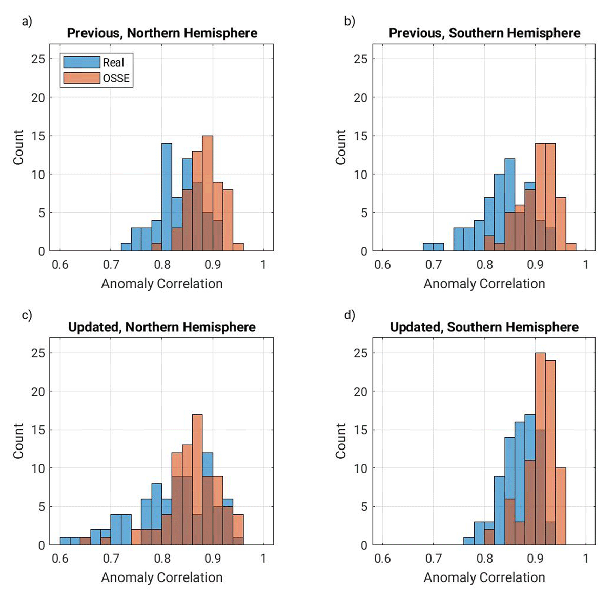
Figure 9
Histogram of 120 hour anomaly correlation of 500 hPa geopotential height for Real (blue) and OSSE (orange). a,b), Previous OSSE, 58 total forecasts July to August; c,d) Updated OSSE, 81 total forecasts July to mid September. a,c) Northern Hemisphere; b,d) Southern Hemisphere.
3.4 Forecast Sensitivity Observation Impact
The GEOS/GSI system includes a forecast sensitivity observation impact (FSOI) tool that employs an adjoint model to estimate observation impacts on a short-term forecast error norm. A moist adjoint has been developed (Halliwell et al., 2014), and a standard choice of error norm is the total wet energy of the 24 hour forecast. The characteristics of the Previous OSSE framework FSOI have been extensively described by Privé and Errico (2019), Privé et al. (2020), and Privé et al. (2021). Figure 10 shows the global net FSOI results compared to real observations for July. August and September 2020 were subject to multiple real observation outages and are thus omitted, although results are similar to July overall. In the previous OSSE framework, the net impacts of the simulated observations were roughly half the magnitude of corresponding real observations, but the relative impact of different types of observing systems was generally well characterized. This reduced impact was deduced to be due to insufficient model error growth in the OSSE framework compared to the real world, resulting in less “work” for the observations to perform.
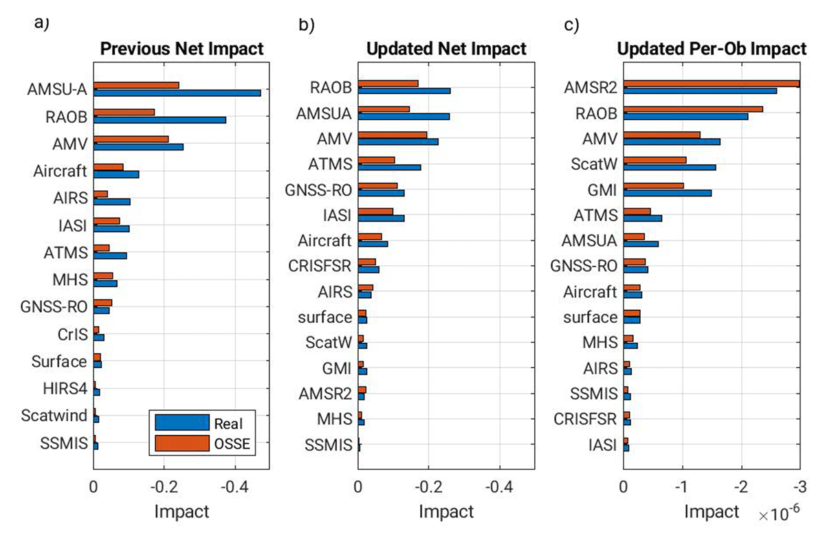
Figure 10
FSOI for global 24 hour total wet energy error norm. 62 total forecasts at 0000 UTC, July–Aug, with numerically unstable solutions omitted. Blue, real observations; red, simulated observations in OSSE framework. a,b) net forecast impact (units) for Previous (a) and Updated (b) frameworks. c) per-observation impacts for Updated framework.
The net FSOI impacts for the Updated simulated observations are closer to real observation impacts than for the Previous OSSE framework, although some data types still have substantially lower impacts in the OSSE. Rawinsonde and ATMS impacts are expected to be somewhat lower in the OSSE due to fewer simulated than real observations. Because of the limited number of model levels, simulated rawinsondes have fewer observations in each profile compared to real profiles, but as seen in Figure 10c, the per-observation impact for rawinsondes is similar in the OSSE to real rawinsondes. ATMS uses a complicated ‘super-obbing’ in the real world that proved very difficult to simulate, and as a result the count of actual ingested simulated ATMS observations is approximately 20% lower than for real ATMS. The anomalously small impacts for AMSU-A types in the Updated framework are consistent across all regions and AMSU-A platforms, and are not well understood, especially considering the excellent matching of AMSU-A counts and observation innovations.
A major change to the global observing system in the Updated framework is the implementation of all-sky radiances for AMSR2, GMI, and MHS. The FSOI net impact estimates for the all-sky data types have low magnitude total global impacts for both the Real and OSSE cases, in part due to relatively small observation counts for these data types. Looking at the per-observation impacts, AMSR2 has the largest per-observation impacts, with good agreement between OSSE and Real. Per-observation impacts for GMI and MHS are weaker in the OSSE than for Real, but are in line with the relative performance of clear-sky radiance types.
4 Observation Impacts for New Instruments
As part of the transition between the Previous and Updated OSSE frameworks, several proposed new instruments were tested in both frameworks. In these experiments, the same dataset for the new instrument was used in addition to the Control observations in each of the OSSE frameworks. Here, the impacts of the proposed instruments are compared between the Previous and Updated OSSE frameworks to show how strongly the impacts depend on the characteristics of the OSSE.
4.1 Geostationary Hyperspectral Infrared (IR)
In preparation for the proposed sounder onboard the Geostationary eXtended Observations (GeoXO) program’s central satellite, McGrath-Spangler et al. (2022) evaluated the potential impact of geostationary hyperspectral infrared (GEO IR) sounders on global numerical weather prediction. Using the Previous OSSE framework, hourly observations were generated for 2960 channels operating from 650 to 2500 cm–1 with a spectral wavenumber resolution of 0.625 cm–1 using the methodology described in Errico et al. (2017). Channel selection was based on an expanded range of the specified Meteosat Third Generation Infrared Sounder (MTG-IRS). Assimilated channels included temperature sounding and water vapor channels, providing atmospheric profiling. A global ring of geostationary satellites was generated based on the GOES-R coverage, relocated to the satellite subpoints of 105°W, 0°, 105°E, and 140°E longitude, consistent with proposed locations of GeoXO’s central satellite, MTG-S, Fengyun-4A, and Himawari-10, respectively. Synthetic errors were not added to the simulated geostationary hyperspectral IR observations. The experiments of McGrath-Spangler et al. (2022) were repeated using the Updated OSSE framework.
First, a comparison of the RTMS analysis error impacts of the GEO IR observations between the Previous OSSE and the Updated OSSE is provided in Figure 11. In this figure, the zonal mean normalized differences in the error show the impact of assimilating geostationary IR sounder radiances on temperature (T), specific humidity (Q), and zonal wind (U) relative to the Control. Temperature and specific humidity are directly impacted by the GEO IR radiances through assimilation of temperature and water vapor sensitive channels. The zonal wind, however, is impacted indirectly through covariances with the directly observed variables (Peubey and McNally, 2009) and benefits from the high temporal resolution possible with a geostationary orbit.
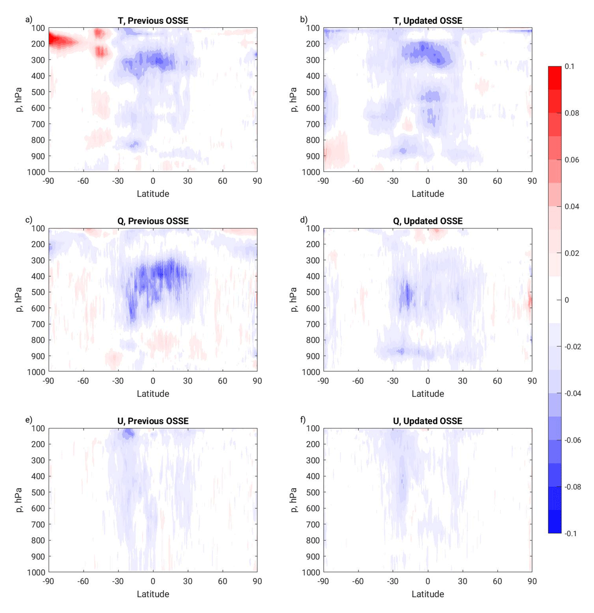
Figure 11
Global fractional difference in RTMS analysis error for the GEO IR experiment vs Control, normalized by the Control analysis error as a function of pressure and latitude for the (left) Previous and (right) Updated OSSE. Shown are the impacts on (top) temperature, (middle) specific humidity, and (bottom) zonal wind. Errors are computed for the months of July and August. Blue and red indicates an improvement and degradation, respectively by the addition of geostationary infrared radiances.
In the Previous OSSE, the temperature impact showed a beneficial impact throughout the tropical troposphere aloft of about 900 hPa. The largest improvement occurring in the tropics is expected because these are the latitudes with the broadest observational coverage by a geostationary orbit. However, there is a degradation south of approximately 30°S associated with an increased error off the west coast of South America (McGrath-Spangler et al., 2022). An even larger temperature degradation exists near the South Polar tropopause, outside the coverage of the assimilated GEO IR satellite observations. Tests showed that this South Polar impact (and all impacts outside the GEO IR observed range) is not directly related to the observations, but is instead a result of model interactions.
With the Updated framework, the strong polar degradation aloft is eliminated and most of the global troposphere is improved by the addition of the observations targeted in these experiments. In addition to the large improvements in the upper tropical troposphere and around 850 hPa, an additional mid-tropospheric region of improvement is present around 10°N in the Updated OSSE. This region corresponds to the areas of increased background temperature error in the Updated framework at the same latitude in Figure 4g. Aloft of 800 hPa over the South Pole, the response is beneficial due to a transference of the information content beyond the latitudes observed by the GEO sounders. At these high latitudes, a small degradation exists above the Antarctic ice and below 800 hPa in the Updated OSSE that was not present in the previous iteration.
The specific humidity is subtly affected by the choice of data assimilation system chosen. In the Previous OSSE, the main benefit exists in the mid-troposphere from between roughly 700 and 300 hPa and equatorward of 30°. A mild degradation below 800 hPa within this latitude range and minor degradations within the extratropical troposphere exist, which is detrimental to the analysis. An examination of the impact in the Updated OSSE reveals a less intense, but more widespread beneficial impact. The lower tropospheric tropics now show a beneficial impact throughout the tropics that is noteworthy due to its co-location with the high water vapor concentrations in this region and their relevance for low-level cloud formation. This region of enhanced beneficial humidity impacts in the Updated framework corresponds to the large increase in background humidity error as seen in Figure 4h. Weaker humidity impacts in the mid-tropospheric tropics in the Updated framework may similarly be related to smaller magnitudes of background error in this region compared to the Previous framework. Additionally, the extratropical degradations are nearly eliminated in the Updated OSSE.
For wind, the Previous OSSE shows benefits mostly within the tropical tropospheric column, but a mild degradation in the extratropics poleward of 30°. The largest improvements are at about 20°S near the tropopause but extend downward to about 800 hPa. In the Updated OSSE, the degradations in the extratropics are nearly eliminated while the tropical benefits are maintained. The largest intensity improvement is retained in the upper troposphere at about 20°S and that extends through the mid-troposphere. Overall, the differences between impacts in the two OSSE frameworks are minimal in the tropics.
A comparison of the relative impact of geostationary IR radiance assimilation on forecast RAMS error is shown in Figure 12. This figure shows the global mean error impacts normalized by the respective Control experiment’s forecast errors, computed for the months of July and August. Shown are the impacts on T, Q, and U. Statistical significance at the 90% level is indicated by stippling.
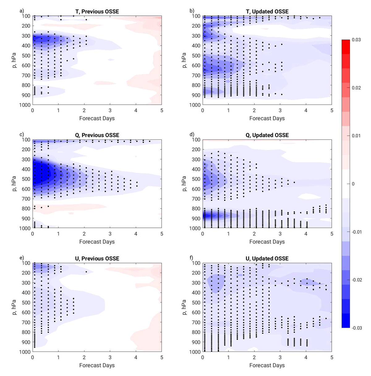
Figure 12
Global fractional difference in RAMS forecast error for the GEO IR experiment vs Control, normalized by the Control forecast error as a function of pressure and forecast time for the (left) Previous and (right) Updated OSSE. Shown are the impacts on (top) temperature, (middle) specific humidity, and (bottom) zonal wind. Errors are computed for the months of July and August. Blue and red indicates an improvement and degradation, respectively, by the addition of geostationary infrared radiances. Stippling indicates significance at the 90% level.
In the Previous OSSE, the temperature impact presented predominantly between 400 and 300 hPa up to the one day forecast with a weaker, beneficial response between 900 and 400 hPa and aloft of 150 hPa. The maximum extent of statistical significance was to 2 days at the higher altitudes. As evaluated in this framework, a small, statistically insignificant degradation was present at about 200 hPa starting from about the 12 h forecast and throughout the troposphere beyond the 4 day forecast. This is consistent with prior work that found that the largest impacts occur during the early forecast period (Privé and Errico, 2013a; Cucurull and Casey, 2021; Privé et al., 2022) and that the impact of the initial condition improvement weakens as model error and chaotic error growth begin to dominate. Tropical forecast improvements are the largest (not shown), with longest duration of significant benefit, with little to no improvement in the Southern Hemisphere extratropics, and weaker, short-lived improvements in the Northern Hemisphere extratropics.
In the Updated OSSE framework, the beneficial impact extends throughout the troposphere and throughout the forecast period with statistical significance extending to nearly the 5 day forecast at the upper levels and approximately 3 days elsewhere. Within the atmospheric column, particular layers of improvement exist with the most intense occurring between 700 and 500 hPa. In this framework, the beneficial impact penetrates deeper into the atmosphere and persists longer with only limited areas of degradation. The extended beneficial impacts of GEO IR on temperature in the Updated framework are due to contributions from both improved impacts in the Southern Hemisphere extratropics and the tropics, where significant beneficial impacts persist into the 2–3 day range (not shown). The improved temperature analysis impacts in the Southern Hemisphere extratropics likely contribute to the longer duration of improved forecast impacts seen in the Updated framework compared to the Previous framework.
Similarly, the impact on water vapor forecasts is affected by the choice of OSSE framework used. In the Previous OSSE framework, the specific humidity is strongly affected between 700 and 300 hPa with a weaker beneficial impact aloft of 300 hPa and near the surface, and a degradation around 800 hPa. The mid-tropospheric improvement and the improvement at 100 hPa are statistically significant until approximately 4 days while the impacts at other levels are for shorter duration. Although an improved mid-tropospheric specific humidity forecast is important for entrainment, the degradation at the height of boundary layer clouds is not ideal. The strong initial impacts that diminish rapidly during the early forecast period are indicative of a model error growth process that acts quickly to eliminate information from the observations, such as moist convection.
In the Updated OSSE (Figure 12d), the impact of assimilating geostationary IR radiances is significantly beneficial throughout the troposphere, up to 200 hPa. The largest improvement occurs at 900 hPa and retains significance throughout the 5 day forecast with the greatest intensity through the 1 day forecast. This beneficial impact in the lower layers at days 3–5 is largely due to improvements in the tropics (not shown). Although a lower intensity mid-tropospheric improvement is also present in the Updated OSSE, the improvement in the lower troposphere, rather than the degradation seen in the Previous OSSE is meaningful for the forecasting of boundary layer clouds, a critical component of the climate system.
In the Previous OSSE framework, there is a weak beneficial impact on the zonal wind forecast throughout the troposphere that is statistically significant until day 2 in the mid-troposphere. After day 3, the forecast impact evolves into a degradation. The degradation is caused by both a convective feedback in the tropics that evolves after day 2, as well as detrimental impacts in the Southern Hemisphere extratropics after the initial 24-hour forecast period (not shown). In the Updated version, the tropospheric zonal wind improvement persists throughout the 5 day forecast with statistical significance continuing almost until day 3 through much of the atmospheric column and until day 5 at certain levels such as at 300 and 750 hPa. The long duration improvement at 300 hPa is consistent with the height of the midlatitude jets, and improvements above 300 hPa have a substantial contribution from the Southern Hemisphere extratropics. While there is still some evidence of a detrimental convective feedback in the tropics in the Updated OSSE, the Southern Hemisphere extratropics retains beneficial impacts through the five-day forecast period, unlike in the Previous OSSE framework.
4.2 GNSS-RO
In this experiment, approximately 100,000 additional GNSS-RO profiles per day are added to the Control case, following the method described in detail in Privé et al. (2022). Here, the Radio Occultation Processing Package operator (ROPP; Culverwell et al. (2015)) was used to generate the simulated observations using 2-dimensional ray tracing techniques below 10 km and 1-dimensional methods at upper levels. The spatiotemporal locations of the simulated RO profiles were based on the locations of actual GNSS-RO observations in 2009, but with 40 days of real observations occurring in a single simulated day. Simulated observation errors were added to the simulated RO profiles with characteristics matching those calibrated for the 2015 GNSS-RO dataset in the Previous OSSE framework. In the Updated OSSE framework, the experiment was repeated using both the same RO dataset as in the Previous OSSE framework and then again with simulated RO errors matching those calibrated for the 2020 GNSS-RO dataset. The two datasets yielded nearly identical results, and the results using the latter dataset are shown here. In this comparison, cycling was performed for the month of July only; forecasts and FSOI were not produced.
Figure 13 compares the zonal mean RTMS analysis error impacts normalized by the respective Control RTMS analysis errors for the 100k RO experiment in the Previous and Updated OSSE frameworks for the month of July. Temperature and specific humidity are shown as these are directly influenced by the RO data. In the Previous OSSE, temperature improvements were seen in the stratosphere and above 500 hPa in the troposphere. However, some degradation of the analysis state was observed poleward of 40°N/S due to ingestion of the additional GNSS-RO data. This was thought to be due to the use of an observation error weighting (R) by the GSI that has a step function form, with lower observation errors poleward of 40 N/S and higher errors in the tropics (Privé et al., 2022). A localized region of low level degradation over Arctic marine areas was also noted and assessed as being a cold bias related to a boundary level inversion near 900 hPa.
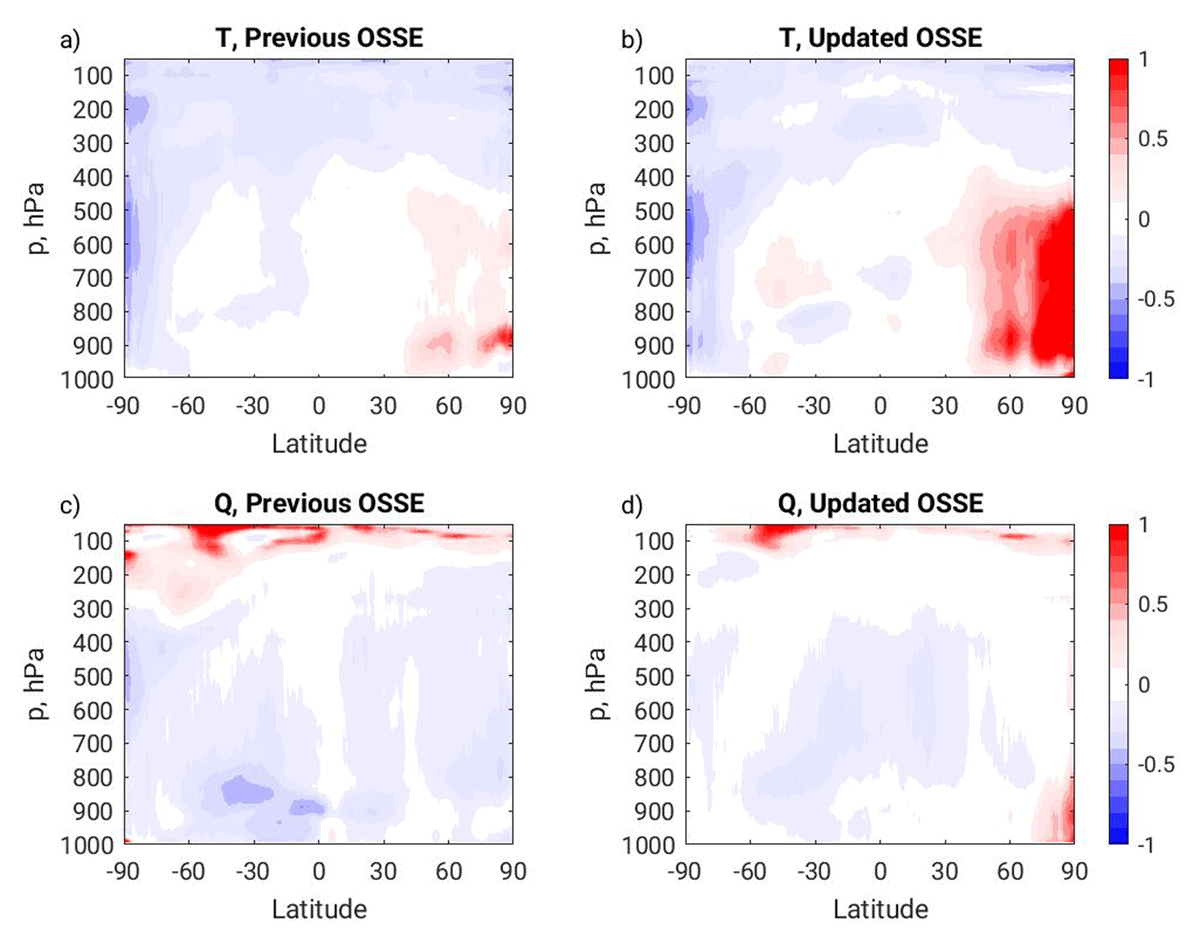
Figure 13
Zonal mean fractional RMS temperature analysis error difference for 100k additional GNSS-RO profile case vs Control, normalized by Control analysis error. Negative values indicate a reduction in analysis error when additional GNSS RO profiles are included. a,b) Temperature; c,d) specific humidity. a,c) Previous OSSE framework. b,d) Updated OSSE framework.
In the Updated OSSE framework, improvements to the analysis due to ingestion of additional RO data are similar to that seen for the Previous framework, but the regions of degradation are amplified, particularly in the Northern Hemisphere. It is noted that there was not a change to the assigned observation error weighting in GSI between the Previous and Updated versions. The strong degradation over Arctic marine surfaces remains in the Updated framework, but now extends up to the mid troposphere. This degradation takes the form of a strong cold bias over marine areas (not shown) below 700 hPa, similar to that seen in the Previous OSSE framework (Privé et al., 2022) but with considerably larger magnitude. Between 700 hPa and 500 hPa, the cold bias is weaker but a large temperature error variance is present. While the temperature increments are clearly detrimental for lower tropospheric RO over the Arctic region, the bending angles show a closer fit for observation minus analysis (O-A) compared to O-B, and the exact cause of this discrepancy is the subject of ongoing investigation.
In the Southern Hemisphere, the RO impacts are fairly similar between the Previous and Updated OSSE. As in the Northern Hemisphere, there is a stronger region of degradation poleward of 40°S in the mid to lower troposphere, indicating that the Updated framework is more sensitive to the assigned observation error weighting than in the Previous framework. Over Antarctica, a region of enhanced beneficial impacts between 900–400 hPa corresponds to a similar area of greater background error in the Updated framework as noted in Figure 4g.
For specific humidity, experiments with the Previous OSSE framework showed beneficial impacts of the additional GNSS-RO observations throughout the troposphere. Degradation of specific humidity in the stratosphere was assessed to be due to poor representation of stratospheric moisture in the OSSE. Improvements to the humidity field were seen in regions where the temperature field was degraded. In the Updated OSSE framework, beneficial impacts of additional GNSS-RO profiles are again observed in the troposphere, but are somewhat weaker overall than in the Previous OSSE. Impacts are most beneficial in the tropics and subtropics, but weaker or even slightly deleterious in polar regions. The change from beneficial to neutral/degradation north of 50°N between the Previous and Updated OSSE versions is likely due to the stronger degradation of the temperature field in the Updated version, as humidity is affected by temperature increments. The lower tropospheric area of degradation of the humidity field near 90°N may also be related to the improvement of the Control background Q field in this region (Figure 4h), as a higher quality background is more likely to be degraded by imperfect observations.
4.3 MISTiC Winds
In this experiment, simulated atmospheric motion vectors for the Midwave Infrared Sounding of Temperature and humidity in a Constellation for Winds (MISTiC Winds) instrument were tested in both OSSE frameworks for the July–August period. The simulated AMVs were generated based on the location of cloud and water vapor features in the NR using probabilistic methods to determine whether an observation was present following the procedure outlined in McCarty et al. (2021). MISTiC radiances were not included in this experiment, and the simulated MISTiC AMVs did not include additional simulated errors for simplicity. A single orbit was selected from the MISTiC constellation of sun-synchronous orbits at 705 km, having local time of ascending node of 1330. Figure 14 compares the zonal mean RTMS zonal wind analysis error of the MISTiC AMV observations normalized by the RTMS Control analysis error in the Previous and Updated OSSE frameworks for the months of July and August, with 4 times daily analyses. The spatial pattern of observation impacts is quite similar, with largest impacts poleward of 60°N/S. The observation impacts have somewhat greater magnitude in the Updated OSSE framework compared to the Previous OSSE, particularly near the poles. This is in line with the overall greater background error for winds in the extratropics seen in Figure 4i for the Updated framework. The background wind error is reduced near the equator in the Updated Control, with a local region of reduction between 100–200 hPa, which may account for the shift of the greatest equatorial MISTiC impact from 100–200 hPa in the Previous framework to 200–300 hPa in the Updated framework.
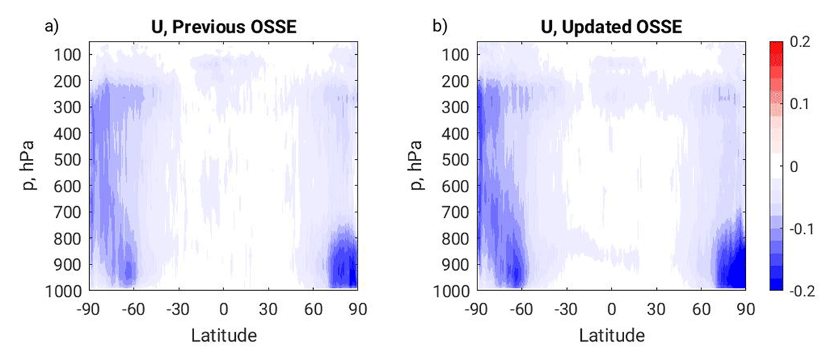
Figure 14
Zonal mean fractional RMS zonal wind analysis error difference for the MiSTIC Wind case vs Control, normalized by Control analysis error, July–Aug. Negative values indicate a reduction in analysis error when MiSTIC winds are included. a) Previous OSSE framework. b) Updated OSSE framework.
The FSOI estimates of global observation impacts on the 24 hour forecast total wet energy error norm are shown for the Control and MISTiC cases in Figure 15. The impact magnitudes for individual types should not be compared between the Previous and Updated OSSE frameworks, it is the relative ranking of impacts that is more pertinent. In the Previous OSSE, MISTiC AMV impacts ranked fourth in net global impact, below combined other AMV types, rawinsondes, and the constellation of AMSU-A instruments. In the Updated OSSE, MISTiC AMVs rank a very close third to rawinsondes and other AMV types, although it is noted in Figure 10 that AMSU-A observations are relatively underweighted in the Updated OSSE. In both the Previous and Updated OSSE frameworks, the impacts of other data types, in particular AMVs, rawinsondes, and AMSU-A, are reduced when MISTiC observations are added, implying a likely degree of redundancy between these data types. While it could be argued that the MISTiC impacts in the Updated OSSE are slightly larger than in the Previous OSSE, which would align with the slightly greater analysis impacts in the Updated framework, the overall FSOI estimate of MISTiC performance is similar in both frameworks.
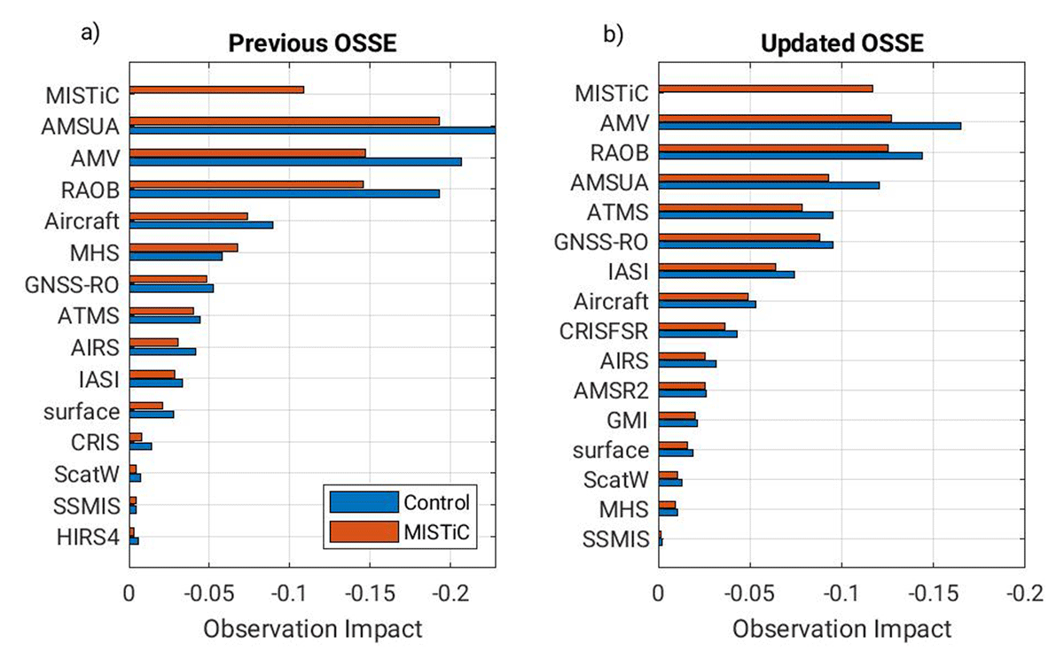
Figure 15
FSOI estimates of observation impact on the 24 hr forecast total wet energy norm. Blue bars, Control; red bars Control + MISTiC winds. a) Previous OSSE framework. b) Updated OSSE framework.
It is notable from Figure 10 that in the OSSE Control, existing AMV types have the largest net impact of any instrument type, while in the Real world, AMVs are ranked third. AMV observations have persistently had an overly large impact in the OSSE framework through multiple changes to the Nature Run, simulated observations, DAS, and forward model (Privé et al. (2013b), Privé and Errico (2019)). Significant changes to the simulated AMV errors and the method of generating AMVs have not lead to a reduction in the relative overestimation of AMV impacts in the OSSE framework over numerous versions of the OSSE.
5 Discussion
Periodic updates of any OSSE framework are required in order to keep up with advancements in both the operational NWP system and the global observing network. Once the operational system overtakes the Nature Run in terms of skill and/or resolution, it is also necessary to upgrade the NR. In this case, the operational GEOS model has not yet reached the high resolution of the NR. However, in the coming years, an increase to the number of vertical levels in the operational GEOS model will necessitate the development of a new NR framework (Privé, 2021).
The main motivation behind the particular choice of GEOS model version used in the Updated OSSE framework was the implementation of a set of major changes to the model physics and dynamics. These model upgrades were expected to increase the model error growth in the OSSE framework by introducing additional differences between the G5NR model and the experiment version of GEOS. This should have the effect of mitigating somewhat the ‘fraternal twin’ situation caused by using similar models for both the NR and the experiment forecasts. Insufficient model error affects every aspect of the OSSE, from the calibration of the simulated observations to the observation impacts on the medium range forecast period.
It is clear from Figure 8 that there is greater forecast error in the Updated OSSE compared to the Previous OSSE framework, particularly in the Tropics and the summer (Northern) Hemisphere. In the Updated OSSE, the Relaxed Arakawa Schubert deep convective parameterization was replaced with a combination of the Greel and Freitas scale-aware deep and congestus parameterization (Freitas et al., 2018) along with the Park and Bretherton shallow convection scheme (Park and Bretherton, 2009). These changes to the convection scheme, along with updates to the radiation scheme and boundary layer schemes, likely play a role in the observed increased forecast error in the Updated framework. The anomaly correlations (Figure 9) similarly show that while the OSSE framework is more skillful than the real data performance of the GEOS/GSI, in the Northern Hemisphere the skill scores for the 5-day forecasts in the Updated framework have a wider spread than in the Previous framework, more closely matching the distribution of forecast skills in the real system. In the Southern Hemisphere extratropics, only the humidity field shows significantly greater forecast error in the Updated compared to Previous OSSE frameworks. Correspondingly, there is not an increased spread of the anomaly correlation scores in the Southern Hemisphere for the Updated system.
The impacts of greater model error are observed in other aspects of the OSSE framework. The background error in the Updated framework Control is generally larger than in the Previous framework (Figure 4). Similarly, the analysis increments in the Updated OSSE are approximately 20% smaller in magnitude compared to the corresponding real data case, while in the Previous OSSE, the Control analysis increments were 30% smaller than the corresponding real case (Privé et al., 2021). The analysis increment can be considered a measure of ‘work’ that is performed by ingestion of the observations, and that is also balanced by the forecast error growth between cycle times. These results can be compared with a much earlier version of the GMAO OSSE wherein the Nature Run was produced using the European Centre for Medium-range Weather Forecast operational model (Errico et al., 2013), where the analysis increments were 5-20% smaller than the corresponding real case. The Updated OSSE can still be considered a ‘fraternal twin’ OSSE, but the degree of twinning has been reduced.
Another beneficial impact of increased model error in the Updated framework is the reduction in the magnitude of simulated observation errors needed to match observation innovation statistics in the real world. When the background error in the OSSE has lower magnitudes than in the real system, the simulated observation errors applied in the OSSE framework to the existing global observation network may be overinflated in compensation. Although previous work (Privé et al. (2013a), Privé et al. (2021)) has shown that FSOI estimates of observation impacts are only modestly affected by changes to the magnitude of simulated observation errors, more realistic representation of observation errors in the OSSE framework is preferred.
The extension of the OSSE simulation period into September in the Updated framework allows the calibration of the simulated observations to be tested. There may be seasonal changes to the climatology of the NR that could affect the count and observation innovation of the simulated observations. The observation validation for the month of September was not as good a match between OSSE and Real as was seen for the months of July and August, however the loss of fidelity was not substantial enough to warrant a recalibration of the observations. A preliminary investigation of the performance of the month of October showed considerably worse validation of the observation characteristics for many data types. It is therefore anticipated that if the OSSE were to be extended into a different season, a recalibration of the probabilistic cloud contamination, AMV locations, and simulated observation errors would be required.
Due to the level of effort required to update the OSSE framework, the OSSE tends to lag behind the progress of the data assimilation system and forward model, as well as the use of a global observing network that may be outdated by several years. This calls into question whether the results of OSSE experiments for proposed new instruments are applicable to the more current NWP system. The use of a fraternal twin OSSE framework can also cast doubt on experimental results. The comparisons of observation experiments shown here use the same simulated observations for the new instruments and the same time period of the NR, so that the synoptics and predictability of the atmosphere are the same. The changes between the experiment results in the Previous and Updated OSSE frameworks are due to the changes to the global observing network, the capabilities of the DAS, and the model forecast skill. Unlike in the real world where a newer forecast model version would be expected to be better than an older version of the same model, the model skill of the forecasts in the Updated framework should be worse than in the Previous OSSE framework because the forecast model is more dissimilar from the NR. However, this greater model error introduces more realism into the OSSE framework and reduces somewhat the problem of twinning.
The FSOI estimates of observation error can be used to calculate a bulk impact by summing the total impact of all observations. In the Previous OSSE framework, the total impact in the OSSE was approximately 60% of the impact in the real system. In the Updated OSSE, the FSOI total impact is more than 70% of the corresponding real system impact. This is due to both a slight increase in the OSSE net FSOI along with a reduction in the net impact of real data with the Updated model and DAS. Some differences in the real system FSOI between the Previous and Updated versions may be due to the differing synoptic situation and predictability of the real atmosphere in 2015 and 2020, while in the OSSE the same period of the NR is used in both the Previous and Updated frameworks. The increase in OSSE net FSOI in the Updated framework may be related to the increase in model error growth for some fields as seen in Figure 4.
Changes to the background error fields can be related to the magnitude and location of observation impacts. An increase in background error between the Previous and Updated frameworks means that there is either (or both) an increase in model error or a change to the global observing network that results in weaker constraint by the observations. When background error increases, there is more opportunity for observations to do beneficial ‘work’.
Some of the changes in observation impact for the proposed new instruments appear to correspond to increases in the Control background error fields. For example, the GEO IR impacts on specific humidity in the lower troposphere are much more beneficial in the Updated framework, particularly in regions where the background humidity error is greatly increased (Figure 4). In the equatorial mid-troposphere however, the background humidity error in the Updated framework is smaller than in the Previous framework, and the GEO IR impacts in this area are weaker in the Updated framework. Similarly, the MISTiC AMV observation impacts are very close in magnitude and location in the Previous and Updated frameworks, with slightly larger fractional analysis impacts (10–12% compared to 8–10% analysis error improvement) in the Updated framework. The wind background error field in the Updated framework is nearly uniformly 5–10% larger than in the Previous Control. As there were no changes to the DAS handling of MISTiC AMVs between OSSE versions, the increased impacts in the Updated framework are expected to be caused largely by the increased model and background errors.
The GEO IR forecast impacts extend further into the forecast period in the Updated framework compared to the Previous framework. The Southern Hemisphere extratropical impacts are particularly influential in terms of improving the global forecast skill in the Updated framework, and appear to be related to the reversal of impacts poleward of 35°S from detrimental in the Previous OSSE to beneficial in the Updated OSSE. This improved performance of GEO IR may be in part due to improvements to the capabilities of the DAS in handling radiance observations or possibly the background error assignments.
For GNSS-RO, the experiment results from the Previous OSSE framework indicated a likely issue with the observation errors assumed by the GSI (‘R matrix’), which has a step-function type form with higher assigned errors in the tropics and a discontinuity at 40°N/S. These assigned errors were not changed in the DAS between the Previous and Updated frameworks, and the regions of degradation poleward of 40° in the lower and mid troposphere are evident in both frameworks. However, the degradation north of 40°N is much more severe in the Updated framework, with a very strong cold bias below 700 hPa and much larger magnitude of analysis error variance from the surface to 500 hPa. This bias appears to be related to a strong temperature inversion over the Arctic marine areas. The enhanced degradation due to additional RO observations in the Updated OSSE framework may be a result of changes to the boundary layer physics parameterizations that could interact poorly with the RO observations in the presence of a strong inversion.
The comparison of observation impacts in light of the differences in model error has implications for the expected observation impacts in future NWP systems. As NWP systems improve, the expectation is that model error will decrease in the future. In the extreme case of a ‘perfect’ model and accompanying ‘perfect’ DAS, with nearly perfect initial conditions, the observations would have very small but non-zero impacts, correcting the growth of the initial condition errors between cycle times. The ultimate goal of improving NWP systems should therefore result in the gradual diminishment of observation impacts purely through the advancement of modeling and DAS skills, assuming that the global observing network remains robust.
These results have demonstrated that using models with greater differences for the Nature Run and forecast experiments in an OSSE results in greater model error growth and overall larger background errors. This has the effect of magnifying the impact of new observing systems, particularly in regions where background error is greater. However, these effects are modest, and the overall distribution and magnitude of observation impacts is similar in the two systems with different degrees of ‘twinning’. Yu et al. (2019) have shown that a purely identical twin OSSE setup may result in incorrect observation impacts, but the comparisons shown here indicate that a range of fraternal twin OSSEs should give robust experimental results, as long as the degree of twinning is well-understood.
Data Accessibility Statement
The dataset on which this paper is based is too large to be retained or publicly archived with available resources. Documentation and methods used to support this study are available from Nikki Privé at NASA GMAO. The G5NR is available for download from a portal at https://gmao.gsfc.nasa.gov/global_mesoscale/7km-G5NR. The codes used to generate simulated observations are available on github at https://github.com/GEOS-ESM/GOWASP.
Acknowledgements
The authors would like to thank Ron Errico (retired) for his longstanding efforts in developing the GMAO OSSE framework, and most recently in implementing the simulated all-sky observation types used in this manuscript. The software for simulating GPSRO observations was provided by the Radio Occultation Processing Package (ROPP) of the Radio Occultation Meteorology (ROM) Satellite Applications Facility (SAF) of EUMETSAT, with the assistance of Sean Healy at ECMWF.
Funding Information
Support for this project was provided by NASA Goddard Space Flight Center (GSFC). Resources supporting this work were provided by the NASA High-End Computing (HEC) Program through the NASA Center for Climate Simulation (NCCS) at GSFC. David Carvalho acknowledges the FCT/MCTES for the financial support to CESAM (UIDP/50017/2020 + UIDB/50017/2020), through national funds.
Competing Interests
The authors have no competing interests to declare.
Author Contributions
NCP calibrated and validated the Updated OSSE, generated the Control synthetic observations, ran the Control and Real validation runs for both the Previous and Updated OSSEs, performed the experiments for the MISTiC Winds and GNSS-RO, and contributed to writing the manuscript. EMS performed the GeoXO experiments and contributed to writing the manuscript. DC developed the methodology for and simulated the MISTiC AMVs. BK assisted with execution of the Previous and Updated MISTiC AMV experiments. IM generated simulated GeoXO radiance data for the Previous OSSE framework. All authors contributed to discussions and editing of the manuscript.