
1 Introduction
Forecasting natural phenomena such as weather cannot be perfect. Knowing the degree of the imperfection (the forecast uncertainty) is always desirable and sometimes vital, for example, in decision-making. A rough estimate of forecast uncertainty can be obtained by comparing forecasts with verifying observations and averaging the forecast-minus-observation statistics over time and space. This simple approach often results in useful estimates. However, the ‘climatological’ estimates can be insufficient if we predict the state of a nonlinear chaotic system like the Earth’s atmosphere, where the forecast uncertainty can vary depending on the weather situation (on the local structure of the atmospheric flow) and the observational coverage.
To allow for a situation-dependent assessment of the forecast uncertainty, a forecast of forecast uncertainty is needed. In probabilistic terms, we have to predict not just the state of the system (in our case, the atmosphere) but also the probability distribution of the unknown true atmospheric state around the forecast. A Monte-Carlo-based approach known as ensemble prediction, in which the probability distribution of the truth is represented by a small number (tens to hundreds) of points in state space (ensemble members), has proven to be both feasible and useful in predicting major features of forecast uncertainty, see, e.g., Leutbecher and Palmer (2008); Wilks (2011) and references therein.
For ensemble prediction to be successful in predicting the forecast uncertainty, ensemble members need to be pseudo-random draws from a probability distribution that is reasonably close to the conditional probability distribution of the truth given the data available prior to the forecast. The most promising approach here is, arguably, to identify all sources of uncertainty that affect the forecast and then stochastically model each of those ‘input’ uncertainties individually. The forecast uncertainty is caused by uncertainties in (i) meteorological observations, (ii) data assimilation techniques, (iii) boundary conditions, and (iv) the forecast model itself. In this study we are concerned with the latter source, the model uncertainty.
1.1 Model uncertainty
A numerical weather prediction model computes the forecast by time stepping. At each time step, the model has on input, typically, the current model state (defined on a spatial grid), and computes the model state at the next time step or, equivalently, computes the forecast tendency, the difference between the next-time-step and the present model states. The model uncertainty is, by definition, the uncertainty in the forecast tendency, e.g. Orrell et al. (2001). Being accumulated and transformed during the time stepping, the uncertainty in the tendency contributes to the uncertainty in the forecast fields.
The model uncertainty is caused by the following imperfections in the forecast model (listed in order of increasing importance).
Atmospheric model’s partial differential equations normally involve a number of simplifications like the neglect of variations (horizontal and vertical) in the gravitational force or the ideal gas law assumption. The model may also omit some processes like chemical reactions or development and impact of electric charges of hydrometeors.
A classical (i.e., based on laws of physics, not a neural network) meteorological forecast model solves a set of time and space-discretized differential equations. The discretization leads to truncation error.
Subgrid-scale processes are accounted for in atmospheric models in an approximate manner. On the one hand, these processes cannot be reproduced by the discretized model equations because the model grid is too coarse. On the other hand, subgrid-scale processes do impact grid-scale fields due to the nonlinearity of physical laws that govern the evolution of the atmosphere. In forecast models, this impact is assessed using simplified sub-models known as physical parametrization schemes. Simplifications (made in these schemes for computational reasons) along with the inherent uncertainty in the unresolved scales lead to uncertainties/errors in physical parametrizations, e.g., Palmer et al. (2005). Note that some processes in the atmosphere (such as turbulence, convection, and gravity waves) can become increasingly resolved by the model equations just by refining the computational grid, that is, by increasing the model’s spatial and temporal resolution. Therefore, these processes can, actually, be regarded as part of truncation error. The respective physical parametrization schemes, thus, attempt to reduce truncation errors while introducing their own (presumably, smaller) errors/uncertainties.
Our focus in this research is on uncertainties/errors in physical parametrizations of subgrid-scale processes.
1.2 Error and uncertainty
At each model time step, nonlinear interactions of the subgrid-scale field xSGS with itself and with the grid-scale field xGS produce a spectrum of combination wavenumbers some of which fall within the resolvable (grid-scale) range. This yields a contribution of the subgrid-scales to the (grid-scale) forecast tendency, see, e.g., Touil et al., 2007, for a formulation of the problem in turbulence theory. Having a perfect model, we could compute this contribution, let it be denoted π(xSGS, xGS). Deterministic physical parametrization schemes, having, by definition, access only to xGS, attempt to assess this impact, producing a physical tendency, P(xGS). The uncertainty in all physical parametrization schemes combined is the difference between P(xGS) and the true physical tendency π(xSGS, xGS).
The subgrid-scale field xSGS is not explicitly defined in the model, therefore it is unknown and even unknowable to the model (to the extent that xSGS is not determined by xGS). Therefore we assume that xSGS is a random field with some conditional probability density p(xSGS | xGS) (we condition on xGS because it is available to the model). This density induces the probability density p(π | xGS). Then, the ideal (best in the mean square sense) deterministic physical tendency is the conditional expectation of the true tendency given the grid-scale field, e.g., Kwasniok (2012); Shutts and Pallarès (2014), , where 𝔼 stands for expectation. It is that a deterministic physical parametrization seeks to approximate by P(xGS). In these terms, it is meaningful to call
the error in the deterministic physical tendency P. However, the deterministic physical tendency is incapable of simulating the variability of π around its conditional mean value ,
(Palmer, 2012). This is the inherent (irreducible) uncertainty in π(xSGS, xGS) given xGS. Then, the full uncertainty is the difference between the error ɛP and the irreducible uncertainty δP:
The irreducible uncertainty δP is especially important in so-called ‘gray zones’, where a process is partly resolved by the model, meaning that a length scale of xSGS is comparable to the grid spacing. In this case, in each grid cell, the grid-scale impact of the subgrid-scale process is, effectively, a sum of a small (and random) number, ν, of random contributions: . With convection, the contributions to the convective tendency are due to individual convective plumes (Plant and Craig, 2008). With boundary-layer turbulence, are due to individual turbulent eddies (Kober and Craig, 2016). Assuming, for presentation purposes, that all are the same in a grid cell and their number ν follows the Poisson distribution, we readily obtain that , where sd denotes standard deviation. This expression shows that the standard deviation (which measures randomness) and the mean value of the grid-scale impact of subgrid-scale processes are comparable to each other in magnitude if , which is the case in a gray zone as discussed above. This makes the irreducible uncertainty in π indeed substantial and implies that it needs to be properly accounted for in ensemble prediction.
It is worth remarking that the irreducible uncertainty δP caused by the randomness of π given xGS is the aleatory (truly random) uncertainty, therefore it cannot be called error. Whereas ɛP is a kind of systematic error (reducible conditional bias), which is caused by imperfections in the physical parametrization schemes. This latter kind of uncertainty due to lack of knowledge is generically called epistemic. Both aleatory and epistemic uncertainties need to be taken into account in building an ensemble prediction scheme. The ideal random physical tendency is a ‘possible true π consistent with the grid-scale field xGS’, that is, a random draw from the probability distribution p(π | xGS). It is reasonable to anticipate that the aleatory part of the uncertainty, being caused by random subgrid noise, should be associated with small spatial and time scales. On the contrary, the epistemic part of the uncertainty caused by systematic and, likely, flow-dependent deficiencies of the physical schemes, may be characterized by larger spatio-temporal scales.
In an ensemble, representing both kinds of uncertainty in physical tendency using pseudo-random spatial fields results in model perturbations introduced at each model time step during the forecast. Techniques that add stochasticity on top of existing deterministic physical parametrization schemes or replace the deterministic schemes with stochastic ones are known as ‘stochastic physics’.
1.3 Existing stochastic physics schemes
The first question is how to represent the aleatory uncertainty in physical tendency in ensemble prediction schemes. We believe that the most sensible way to address this question is to build intrinsically stochastic (rather than traditional deterministic) parametrization schemes. Research in this direction is underway, see Plant and Craig (2008); Dorrestijn et al. (2013); Sakradzija et al. (2015); Hirt et al. (2019); Machulskaya and Seifert (2019); Clark et al. (2021) and others. The second question is how to represent the epistemic uncertainty in physical tendency produced either by a deterministic or a stochastic physical parametrization scheme.
We state that, on the one hand, stochastic parametrizations have not yet replaced deterministic ones. So we still need techniques to represent uncertainties in deterministic physical parametrizations. Ad-hoc approaches are in wide use here. On the other hand, stochastic parametrizations are not going to be devoid of epistemic uncertainties either. To represent those uncertainties, we will, most likely, resort to ad-hoc schemes, too. Our focus in this research is on ad-hoc model perturbation schemes.
Currently, the two most popular ad-hoc techniques to represent uncertainties in physical parametrizations are Stochastically Perturbed Parametrization Tendencies (SPPT, Buizza et al., 1999; Leutbecher et al., 2017) and Stochastically Perturbed Parametrizations (SPP, Ollinaho et al., 2017). SPPT generates model perturbations relying on the assumption that the magnitude of the error in the physical tendency is proportional to the magnitude of the physical tendency itself. There is also a flavor of SPPT called iSPPT in which tendencies from different physical parametrizations are perturbed independently (Christensen et al., 2017). SPPT has proven to be very useful in practical ensemble prediction schemes despite its lack of physical consistency: it does not respect conservation laws because it perturbs tendencies without modifying fluxes, see Leutbecher et al. (2017), Lang et al. (2021), and references therein.
In SPP, selected parametric and structural elements of the model’s parametrization schemes are made spatio-temporal random fields rather than fixed numbers and fixed choices. Advantages of SPP include (i) reliance on expert knowledge to select perturbed elements and design probability distributions, (ii) internal consistency of the resulting numerical scheme and conservation properties, and (iii) capability of generating significant spread in the ensemble (Lang et al., 2021; McTaggart-Cowan et al., 2022). The disadvantages of SPP are more conceptual. First, it accounts only for uncertainties that can be captured by perturbing the specific parametrization schemes used in the forecast model in question. Given the inevitably simplified nature of many parametrization schemes, the resulting tendency perturbations may not explore some relevant directions in phase space. Second, it is hard to even suggest how, say, parameter-perturbation probability distributions can be objectively justified. The reason is that parameters (and structural elements) of parametrization schemes may have no counterparts in nature (there is no ‘diffusion coefficient’ in nature) and even in a high-resolution model used as a proxy to the truth. Besides, both SPPT and SPP can lead to biases, see, e.g., Leutbecher et al. (2017) and Bouttier et al. (2022), respectively.
We selected SPPT (described in more detail in section 2.1) as a starting point for our development in this study because it attempts to do exactly what is needed to represent uncertainty in physical parametrizations: it perturbs the physical tendency (see above section 1.2).
In this study, we analyze limitations of SPPT and build a technique that attempts to address those limitations. The new scheme termed Additive Model-uncertainty perturbations scaled by Physical Tendencies (AMPT) is tested in numerical experiments with a convective-scale ensemble prediction system.
2 Methodology
In this section, we review SPPT and introduce a new approach to generation of model-uncertainty perturbations. The new AMPT scheme builds on SPPT and attempts to avoid/relax some of the deficiencies of SPPT. AMPT is applied to both atmosphere and soil.
2.1 Background on SPPT and notation
To facilitate the presentation of AMPT, we first outline SPPT (Leutbecher et al., 2017). By we denote the vector-valued physical tendency (the net physical tendency, that is, generated by all physical parametrizations combined) at the spatial grid point with the Cartesian horizontal coordinates (x, y), the vertical coordinate ζ, and the forecast time t. Here Pi(x, y, ζ, t) is the component of P(x, y, ζ, t) in the i-th model field (variable) Xi, and nfields is the number of model fields selected to be perturbed (most often, temperature, winds, and humidity, e.g., Christensen et al., 2017).
In SPPT, the perturbed physical tendency P* is postulated to be
where ξ(x, y, t) is the zero-mean and unit-variance spatio-temporal random field and κ the scalar (i.e. the same for all model variables) parameter that controls the magnitude of the perturbation. For stability reasons (to avoid sign reversal of the physical tendency, see, e.g., Leutbecher et al., 2017), the support of the probability distribution of κ ξ(x, y, t) is limited to the segment [–1,1] so that
This constraint limits the magnitude of perturbations in SPPT.
From Eq. (4), the perturbation of the physical tendency in SPPT is seen to be multiplicative with respect to the model physical tendency:
Here and elsewhere Δ denotes a perturbation.
2.2 Motivation
The following deficiencies of SPPT led us to propose the new approach.
In SPPT, perturbations are large (small) when and where the physical parametrizations generate a large (small) physical tendency P. This formulation gives rise to a meaningful scaling of perturbations in situations when the model predicts a high or moderate intensity of subgrid-scale processes and produces a large or moderate physical tendency. However, it cannot cover situations in which the physical tendency appears to be small or even zero whereas the model uncertainty is, in fact, large. This may occur if, for example, in a grid cell, convection is initiated in nature whilst the convective parametrization fails to be activated (note that in this case switching to iSPPT would not help either).
Equation (6) implies that the multivariate perturbation vector ΔP(x, y, ζ, t) is strictly proportional to the physical tendency vector P(x, y, ζ, t). As noted by Leutbecher et al. (2017), this implies that SPPT tacitly assumes that only the magnitude of the vector P is in error and not its direction, which is highly unlikely. In other words, SPPT ‘assumes’ that the ratios of the physical tendencies in different variables i and j at the same point (x, y, ζ, t) are error-free. As a consequence, the SPPT perturbations (and thus the assumed model uncertainties) are perfectly (100%) correlated or perfectly (–100%) anticorrelated for any pair of model variables, which is not realistic.
Indeed, from Eq. (6) written component-wise, we have ΔPi = κ ξ Pi, where κ is a positive constant and 𝔼 ξ = 0. This implies that 𝔼 (ΔPi | Pi) = 0, and Cov (ΔPi, ΔPj | Pi, Pj) = 𝔼 (ΔPi ΔPj | Pi, Pj) = κ2(sd ξ)2 PiPj (where Cov stands for covariance). Taking into account that sd (ΔPi | Pi)= κ |Pi| sd ξ and sd (ΔPj | Pj) = κ |Pj| sd ξ, the correlation, that is, the covariance normalized by the product of the two standard deviations, becomes Corr (ΔPi, ΔPj | Pi, Pj) = ±1.
Similarly (and also noted by Leutbecher et al., 2017), since the SPPT random pattern ξ(x, y, t) does not depend on the vertical coordinate, the SPPT perturbations are perfectly coherent (correlated) for all variables at all levels in a vertical column, which again is unrealistic.
Moreover, it has appeared that for SPPT to give rise to a significant spread in the ensemble, the length and time scales need to be really large for convective-scale models. E.g., in Maurer et al. (2014), the tuned length and time scales in the 2.2-km resolution COSMO model were as large as 500 km and 6 h, respectively. This implies that the above unphysical ±100% correlation of SPPT perturbations approximately holds for all model variables in huge 4D volumes spanning the whole atmosphere in the vertical, hundreds of kilometers in the horizontal, and hours of forecast time.
In some models, with their specific configurations of model perturbation schemes, SPPT appeared to generate not enough spread in ensemble forecasts, preventing them from producing reliable probabilistic forecasts, see e.g. Christensen et al. (2017); Frogner et al. (2022). One possible reason for that is the limitation on the magnitude of perturbation, Eq. (5).
With iSPPT (Christensen et al., 2017), the above points 1–3 pertain to the tendency due to a single parametrization scheme. iSPPT alleviates weak points 4–5, allowing for smaller spatial scales of the random pattern and having the capability to generate a somewhat larger spread in the ensemble than SPPT (Wastl et al., 2019; Christensen et al., 2017).
For completeness, it is worth mentioning that in developing AMPT we did not aim at alleviating SPPT’s lack of physical consistency.
2.3 Approach
In AMPT, we propose to address the above deficiencies of SPPT as follows.
2.3.1 Univariate AMPT design
We rely on the SPPT’s assumption that the standard deviation of the model-uncertainty perturbation ΔXi = ΔPi is proportional to the modulus of its respective physical tendency, sd(ΔXi | Pi) = κ |Pi|. In AMPT, we define this dependency to be more general than just point-wise, postulating sd(ΔXi | Pi) to be proportional to an area-averaged |Pi|. This allows AMPT to generate non-zero perturbations even at grid points with zero physical tendency — if there are nearby points with non-zero physical tendency. Theoretically, this approach can be justified as follows.
Consider the unknown true model-uncertainty field ɛi(r) (where r is the spatio-temporal coordinate vector (x, y, ζ, t)). Assume that ɛi(r) can be modeled as a random field with zero mean and the unknown spatially variable standard deviation σi(r). In these settings, SPPT, effectively, estimates σi(r) as κ |Pi(r)|, see Eq. (6), that is, the only predictor to estimate σi at the point r in space and time is the physical tendency at the same point. We propose to acknowledge that |Pi(r)| is a noisy ‘observation’ of the true model-uncertainty standard deviation σi(r) and therefore it is worth looking for other predictors, i.e., other data that can contain information on σi(r). In AMPT, we hypothesize that these additional relevant data are values of the absolute physical tendency in the vicinity of the spatio-temporal point in question r. Linearly combining these noisy data, we obtain the AMPT’s estimate of the unknown σi(r) given the known field |Pi(.)|:
where Wi(r, r′) is a weighting function that determines the contribution of the absolute physical tendency, |Pi|, evaluated at the grid point r′ to the estimate of the model-error standard deviation, , evaluated at the grid point r and the integral is over the model domain (and, possibly, over model time as well). With the simplifying assumption that the weighting function is homogeneous, Wi(r, r′) = wi(r – r′), we rewrite Eq. (7) as
where ,
is the local-area averaged absolute physical tendency (we will call it the scaling physical tendency), and is the averaging kernel such that .
Having estimated σi(r), we can simulate the model uncertainty as
where ξi(r) is a zero-mean and unit-variance Gaussian random field postulated to be stationary in space and time. Its spatio-temporal correlations are discussed below in section 2.3.4. Spatial (and temporal) non-stationarity of the model-uncertainty field ɛi defined by Eq. (10) comes from variability in the scaling physical tendency . Non-Gaussianity of the model-uncertainty field comes from the randomness of .
2.3.2 Scaling physical tendency
Technically, with the gridded fields, the integral in Eq. (9) is replaced with a sum. Given the layered structure of the atmosphere, we perform the averaging in the horizontal only:
where (xq, yr) is the horizontal grid point, i (we recall) labels the model variable, and wqr are the averaging weights. The latter are specified to be non-zero only inside the averaging area , where Ai is the half-size of the averaging area (the averaging length scale) in both x and y directions. For simplicity and due to a lack of knowledge on the spatial structure of uncertainties associated with as ‘observations’ on σi(x, y, ζ, t) we adopt the simplest design: the weights wqr are equal to each other within the averaging area and normalized so that for any x,y, we have . In the context of limited area modeling, if the point (x,y), where is evaluated, is near the model’s boundary, Ai is reduced so that the averaging area is still a square and is within the model domain.
If Ai is greater than the size of the domain, the averaging is performed over the whole domain so that is the same for all grid points in the horizontal. This is how we computed the scaling physical tendency for atmospheric temperature, winds, and soil temperature. For less Gaussian fields such as humidity and soil moisture, is computed by averaging over a significantly smaller moving window centered at the grid point in question (see section 3 for details). It is worth noting that dependence of on model time t is essential. The reason is that during the forecast, the mean magnitude of physical tendency may undergo significant variations due to a passage of a front or a convective system, changes in convection, etc.
2.3.3 Multivariate and 3D aspects
First, we allow in AMPT not only for errors in the modulus of the vector P but also for errors in the direction of P. We do so by introducing independent driving random fields ξi for different model variables Xi (see Eq. (10)). Though purely uncorrelated perturbations are unphysical, we rely on the forecast model to introduce physically meaningful relationships between the variables during its adaptation to the model perturbations. Since the magnitude of the perturbation at each model time step is small compared with the natural variability,1 the adaptation is expected to go smoothly.
Second, to get rid of the perfect coherency of the perturbations in the vertical, we switch from the 3D random pattern ξ(x, y, t) in SPPT to the 4D random fields ξi(x, y, ζ, t) in AMPT.
Third, the perturbation-magnitude multiplier κi is variable-specific in AMPT.
2.3.4 Length scales and perturbation magnitudes
Let us assess the horizontal length scale of the SPPT perturbation field, see Eq. (6). To this end, with fixed ζ and t, suppose that the physical tendency Pi(x, y, ζ, t) is a stationary (homogeneous) and isotropic random field as a function of x, y. Let its correlation function be denoted as CP(r), where r is the horizontal distance. Since the random pattern ξ(x, y, t) is stationary, isotropic, and independent of Pi by construction, the horizontal correlation function of the SPPT perturbation field ΔSPPT is , where Cξ(r) is the correlation function of ξ. Assuming, further, that Cξ (r) and CP(r) are twice differentiable, we obtain the differential length scale (e.g., Monin and Yaglom, 2013) of the perturbation field as . Since and , we obtain
where and LP are the differential length scales of the random pattern ξ and the physical tendency P, respectively.
As we noted in item 4 of section 2.2, the optimally tuned length scale of the SPPT random pattern in convective-scale applications appears to be much greater than the respective scales of natural variability. In terms of the differential length scales, we may therefore conclude that . Then, Eq. (12) implies that . Since it is plausible that the optimally tuned approximates the unknown model-uncertainty length scale Lɛ, we obtain
In AMPT, the random pattern ξ multiplies the scaling physical tendency so that
where is the differential length scale of . Since is a spatially smoothed version of |P|, . Therefore, for the length scale of the AMPT perturbation to be close to LP, we have to make , that is, much smaller than in SPPT. The optimally tuned length scales of the AMPT random patterns are given in section 3 (they, indeed, appeared to be an order of magnitude smaller than their SPPT counterparts).
As for the AMPT magnitude multipliers κi, the non-local dependence of the scaling physical tendency on the modulus of the unperturbed physical tendency (Eqs. (9) and (11)) suggests that κi do not need to obey the SPPT’s strict upper limit on the magnitude multiplier, Eq. (5). This allows AMPT to cause greater spread than SPPT in the ensemble if needed.
2.3.5 Further details
The rest of the Methodology section is organized as follows. Details on AMPT perturbations for specific model fields are given below in section 2.4. The Stochastic Pattern Generator (SPG, Tsyrulnikov and Gayfulin, 2017) is outlined in section 2.5. Section 2.6 explains how SPG fields are mapped from the SPG domain onto the model domain. In section 2.7 we briefly discuss stability, conservation properties of the new scheme, possible biases due to nonlinearity of the forecast model, and explain the terminology according to which we call SPPT perturbations multiplicative and AMPT perturbations additive.
2.4 Treatment of specific model fields
In the atmosphere, we experimented with perturbations of the 3D fields of temperature T, pressure p, horizontal wind components u, v, and specific humidity qv. We also tried perturbing cloud ice and cloud water but found that those perturbations had little overall impact, so we abandoned them. In the soil, we perturbed 3D fields of soil temperature and soil moisture.
2.4.1 Atmospheric temperature, pressure, and winds
Independent perturbations of T, u, v are computed following Eq. (10). The pressure perturbation Δp is computed from ΔT by integrating the hydrostatic equation (in which Δqv is neglected as a small contribution to a small perturbation) assuming zero pressure perturbation at the top of the model domain.
As for wind perturbations, we note that theoretically, it is ‘better’ to rely on mutually uncorrelated random stream function and velocity potential perturbation fields —rather than on mutually uncorrelated u and v (i.e., zonal and meridional wind) perturbation fields. The reason is that the former approach allows for isotropic vector-wind perturbations (Monin and Yaglom, 2013, section 12.3), unlike the latter approach. However, in practical terms, we were not able to identify any practically significant flaw in the vector field composed of two independent u and v perturbation fields. For this reason and due to the lack of evidence on the actual structure of model uncertainties, we stick to the simpler formulation of AMPT with mutually independent Δu(x, y, ζ, t) and Δv(x, y, ζ, t) in this study.
2.4.2 Humidity
The salient difference of humidity qv from T, u, v is that qv has a narrow range of values (from zero to saturation or somewhat higher than saturation). The range of qv is narrow in the sense that it is comparable to the standard deviation of the natural variability in qv. To make sure that the AMPT-perturbed qv is within this range (i.e., from zero to saturation) and does not directly introduce any bias into the model, we modify the above formulation of AMPT. Specifically, we employ a kind of ‘perturbation symmetrization’ as follows. Consider a grid point s and model time t, where and when the unperturbed specific humidity is qv(s, t). We compute the tentative perturbation Δqv(s, t) following Eq. (10) and then symmetrically truncate it at ±c, where c = min(qv(s, t), qsat(s, t) – qv(s, t)) and qsat(s, t) is the saturated specific humidity. Due to the truncation, the perturbed is, first, within the admissible range from 0 to qsat(s, t) and second, as the truncation is symmetric, no bias is directly introduced: (which would not be the case if we just truncated at 0 and qsat(s, t)).
2.4.3 Soil fields
In the land (soil) model, tendencies of two model fields are perturbed: soil temperature Tso and soil moisture (more specifically, soil water content Wso per unit area within the soil layer in question). Compared with the atmospheric AMPT, the differences in the treatment of the soil fields are the following.
The scaling tendencies and are computed by averaging the total tendency, assuming that all processes in the soil are modeled with substantial uncertainty.
The averaging in Eq. (11) is performed over land only.
The perturbation patterns in the soil, and , used to generate perturbations following Eq. (10) are three-dimensional (not four-dimensional as in the atmosphere).
Whole-domain averaging is used to compute the scaling physical tendency . Local-area averaging (i.e., with the averaging length scale much smaller than the domain size) is employed to compute the scaling physical tendency . This choice is motivated by higher variability/non-Gaussianity of soil moisture compared to soil temperature (not shown).
The perturbed Wso is truncated to ensure that the volumetric soil water content ηso is between the wilting-point ηwp and field capacity ηfc:
where Z = 1, 2, …, nZ labels the soil layer, ΔZ is the thickness of the Z-th layer, and nZ is the number of layers.
2.4.4 Initial soil perturbations
In the soil, processes have much longer time scales than in the atmosphere, therefore the role of model perturbations can be revealed only in long-range forecasts or in cycled systems. Dealing in this study with short-range forecasts without cycling and having an under-dispersive ensemble of initial conditions, we had to develop a generator of initial Tso and Wso perturbations.
The initial soil temperature perturbation is specified as
where is the external magnitude parameter, is the vertical-decay external parameter, Z = 0, 1, …, nZ (with Z = 0 denoting the so-called surface temperature and Z = 1, …, nZ labeling the soil layers), and ξ(x, y) is the 2D pseudo-random field. Note that the random pattern ξ is the same for all soil layers, whilst the magnitude of the perturbation exponentially decreases downwards.
With the soil moisture Wso, the technique (inspired by Schraff et al., 2016) is to perturb the Soil Moisture Index
as follows:
where is the magnitude parameter, is the vertical-decay parameter, and Z = 1, 2, …, nZ. If at a grid point, the perturbed S appears to lie outside the meaningful range [0,1], the perturbation ΔS is truncated accordingly. Using Eqs. (17) and (15), we finally convert the perturbation ΔS(x, y, Z) into the perturbation of Wso:
2.5 Stochastic pattern generator (SPG)
In this study, we rely on the limited-area Stochastic Pattern Generator (SPG) developed by (Tsyrulnikov and Gayfulin, 2017) to generate independent four-dimensional spatio-temporal pseudo-random fields ξi needed by AMPT, see Eq. (10). Each ξi is computed by solving the stochastic pseudo-differential equation
Here x, y, z are the SPG-space spatial coordinates, is the 3D Laplacian, α(t, x, y, z) is the Gaussian white noise, and λ, U, σ are the parameters. λ determines the spatial scale of ξ. Given λ, the characteristic velocity U determines the time scale of ξ. Given λ and U, the parameter σ determines the variance of ξ and is selected to ensure that sd ξ = 1. The computational domain is the cube of size 2π and periodic boundary conditions in all three dimensions.
The design of Eq. (20) (note the third order of the equation in time and the square root of the negated and shifted Laplacian) is dictated by two requirements:
The solution ξ satisfies the so-called proportionality of scales property (Tsyroulnikov, 2001). The meaning of this property is the following. For any t, let us expand ξ in Fourier series in space: , where are the spatial wavenumbers and are the Fourier coefficients. Then Eq. (20) decouples into a series of ordinary stochastic differential equations for the random processes . The proportionality of scales means that for a large total wavenumber , the time scale of the process is proportional to its spatial scale , a property often possessed by natural spatio-temporal processes.
The spatial spectra of ξ should be convergent, that is, the process variance should be finite in the space-continuous case and thus should be bounded above as the spatial resolution increases in the space-discrete case.
The solution to Eq. (20) is a zero-mean and unit-variance homogeneous (stationary in time and space) 4D random field, which has ‘nice’ spatio-temporal correlations: the shape of the correlation function is the same along any direction in the 4D space (thus, including spatial and temporal correlations). This universal correlation function belongs to the very popular in spatial statistics Matérn class, see (Tsyrulnikov and Gayfulin, 2017) for details.
Since the SPG computational domain is the cube whereas the limited-area-model domain can be approximated by a rectangular parallelepiped, we use the anisotropic Laplacian instead of in Eq. (20):
Here γ is the aspect ratio of the model domain in the horizontal and δ controls the length scale along the z axis.
The SPG internal parameters (for the model variable labeled by i) λi and δi are computed from the respective horizontal and vertical length scales, Li and Hi, which are SPG external parameters (this is done by taking advantage of the known correlation functions of the 4D SPG field in space and time). The time scale is , where U is the above characteristic velocity (another external parameter).
With each realization of the driving white noise α, the solution to Eq. (20) is computed in 3D Fourier space using the backward Euler finite difference scheme in time. Once per model time, the solution is converted to physical space (using the 3D inverse fast Fourier transform, FFT). The resulting physical-space random pattern ξ(t,x,y,z) is then mapped onto the model domain and used to compute model perturbations (according to Eq. (10)) for the next model time interval. Avoiding the application of the inverse Fourier transform every time step significantly reduces the computational cost of the numerical scheme. is selected to be a few times less than the time scale of the process, .
SPG can also generate 3D fields ξ(t, x, y) and ξ(x, y, z) as well as 2D fields ξ(x, y).
2.6 Mapping fields from SPG grid to model grid
In each of the three spatial dimensions, to avoid significant unphysical correlations in ξi between the opposite sides of the model domain due to the periodicity of the SPG domain, a segment of length 2Li in the SPG domain is, first, discarded. Then, the rest of the SPG domain (the ‘working domain’) is mapped onto the model domain, where the field is interpolated to the model grid points. In the horizontal, the mapping is piecewise linear. In the vertical, two options were explored.
With Option 1, the mapping z ⟼ ζ (where ζ is the model’s vertical coordinate) is piecewise linear (just as in the horizontal) so that in the model space, the resulting field is stationary (homogeneous) in the vertical as a function of ζ.
With Option 2, a non-stationarity (inhomogeneity) in the vertical is introduced. Specifically, we assume that the model vertical levels are unevenly positioned by the model designer to account for the variable vertical length scale of the model fields. Say, in the planetary boundary layer, the model levels are dense, reflecting shallower meteorological structures (and thus shorter vertical length scales) than in the troposphere and stratosphere, where the vertical grid is much coarser because the vertical length scales are greater.
To obtain the same vertical inhomogeneity in AMPT perturbations interpolated to the model grid, we employ a mapping that is linear from the SPG coordinate z to the model vertical (continuous) ‘computational’ coordinate defined to be equal to at the model level . With this mapping, the correlations between all adjacent model grid points in the vertical are the same (due to stationarity of the SPG field as a function of z). As a result, in model space, the vertical correlation falls to the same value at short vertical distances in the boundary layer (because the model grid is dense there) and at longer vertical distances above the boundary layer (where the model grid is coarser) thus implying the desired inhomogeneity in the vertical.
2.7 Properties of AMPT
2.7.1 Stability
Stochastic-dynamic systems in which the magnitude of random forcing depends on the current state of the system and the forcing (perturbation) is time-correlated, can be unstable due to a positive feedback loop. Indeed, a deviation of the model state from its mean value may result in a greater forcing, which may lead to an even greater deviation of the state from the mean, and so on until ‘explosion’. To break this vicious circle, we considered two strategies.
A technically simpler one, which we adopted in this study, is to update the scaling tendency not at every time step but less frequently, once per model time during the forecast, where is an external parameter defined below in section 3.
A somewhat more involved but potentially more powerful approach (which we left for future research) is to calculate the scaling physical tendency from the unperturbed (control) model run, xcontrol, let us denote it (where i labels the model variable, s is the spatial grid point, and t is time). The scaling physical tendency, being a moving average of the modulus of the physical tendency, is a smooth field, so can be stored during the control run in a file on a coarse spatio-temporal grid (meaning that this should be feasible in terms of required computer resources). Then, can be used to compute AMPT perturbations for all ensemble members. By construction, this device will destroy the harmful positive feedback loop. We remark that taking fields from the control run to make model perturbations state-dependent can be used to prevent instabilities not only with AMPT but with other techniques as well.
However, as noted by an anonymous reviewer, this technique cannot be applied to long-range predictions where ensemble members may diverge from the unperturbed member to the extent that the physical tendency produced by the latter becomes irrelevant for the former. Another caveat is that an application of that technique to an operational ensemble prediction system will require that the unperturbed member be computed somewhat earlier than the rest of the ensemble.
Another promising approach is to perturb fluxes instead of prognostic fields, as discussed in section 2.7.2.
2.7.2 Conservation properties
Neither SPPT nor AMPT respects local conservation laws. The reason is that in both SPPT and AMPT, the model fields are perturbed whereas the fluxes are not. Switching from perturbing state variables to perturbing fluxes (as done by Van Ginderachter et al., 2020, for deep convection), including boundary fluxes, would solve the problem. However, a purely flux-based model perturbation scheme aimed to represent uncertainties in multiple physical parametrizations remains to be built and tested, which is beyond the scope of this study.
2.7.3 Biases
It is well known and easy to understand that feeding a nonlinear system with an unbiased signal can lead to a biased system output. Biases can appear even in a linear system if it is perturbed in a multiplicative way, like in SPPT. Bouttier et al. (2012, Figures 3 and 5) and Leutbecher et al. (2017, Fig. A1(a)) found that in their systems, SPPT led to the drying of the atmosphere and reduced precipitation. In experiments by Romine et al. (2014) the atmosphere also became too dry due to SPPT (their Figure 5 and 8) but that was associated with an increase in precipitation (their Figure 9). One possible reason that led to different outcomes in those studies is the impact of the supersaturation limiter (which nullifies temperature and humidity perturbations at the grid points where the water vapor is saturated or super-saturated). We experimentally study forecast biases induced by various configurations of AMPT and compare them with forecast biases induced by SPPT in section 4.
2.7.4 Additive vs multiplicative model perturbations
In Appendix A, we discuss why SPPT perturbations are multiplicative and why we call AMPT perturbations additive. We show that AMPT perturbations are truly additive in the setting when the scaling physical tendency is taken from the control run (this option was discussed in section 2.7.1).
In numerical experiments presented below, the model perturbation scheme is an approximation to the setting in which the scaling physical tendency is completely decoupled from the current model state. The coupling is only relaxed by updating the scaling physical tendency much less frequently than every model time step (see sections 2.7.1 and 3). In this regime, AMPT perturbations are not multiplicative but not yet fully additive. Nevertheless, with some abuse of terminology, we call them additive bearing in mind the above scheme with the scaling physical tendency taken from the unperturbed model run.
3 Experimental Settings
The program code of AMPT was built into the limited-area non-hydrostatic COSMO model (Baldauf et al., 2011), which has both atmospheric and soil prediction modules. The model was, in turn, embedded in a limited-area ensemble prediction system. The AMPT-generated model perturbations along with an ensemble of initial and lateral-boundary conditions allowed us to compute (and verify) ensemble forecasts. The goal was to assess the effect of AMPT on deterministic and probabilistic forecasts and compare it with the effect of SPPT perturbations.
The COSMO model (version 5.01) was used in the convection-permitting configuration with a horizontal grid spacing of 2.2 km, 172*132 grid points in the horizontal, and 50 levels in the vertical. The model integration time step was 20 s. The model’s vertical coordinate was the height-based hybrid (Gal-Chen) coordinate (Gal-Chen and Somerville, 1975).
The ensemble prediction system used in this study was COSMO-Ru2-EPS (Montani et al., 2014; Astakhova et al., 2015), which was developed within the FROST-2014 international project (Kiktev et al., 2017) and the CORSO priority project of the COnsortium for Small-scale MOdeling (COSMO) (Rivin et al., 2018). The ensemble size was 10. COSMO-Ru2-EPS performed a dynamical downscaling of the forecasts of the driving COSMO-S14-EPS system developed by the Italian meteorological service ARPAE-SIMC (Montani et al., 2014). Thus, both initial and lateral boundary conditions for the control forecast and ensemble members were provided by COSMO-S14-EPS, which had a horizontal grid spacing of 7 km and 40 vertical levels. COSMO-S14-EPS was a clone of the consortium ensemble prediction system COSMO-LEPS (Montani et al., 2011) with a smaller ensemble size.
The model domain is shown in Figure 1. Note the complexity of the area, which contains high mountains along with the adjoining valleys and sea. The center of the domain is located nearly at 44°N, 40°E. The climate at the sea level is humid subtropical. Numerical experiments were carried out in this study mostly for the winter-spring season: in February and March, for which we had access to all data needed to run and verify ensemble forecasts. Some sensitivity experiments were also conducted for May cases.
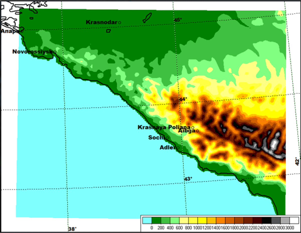
Figure 1
Model domain and orography.
The following AMPT parameters were selected for numerical experiments. The horizontal length scale Li of the SPG driving random fields ξi (where i labels the perturbed fields) was tuned to be 50 km (i.e., 20–25 horizontal mesh sizes) for T, u, v and 35 km for qv. The vertical length scale Hi was about 3 km for T, u, v and about 2 km for humidity.
The characteristic velocity U = 15 m/s was selected from the physically meaningful interval of 10–20 m/s.
After some experimentation, the (dimensionless) model-uncertainty magnitude multipliers κi were specified as 0.75 for T, u, v, Tso, Wso and 0.5 for qv.
The length scale Ai of averaging the absolute physical tendency (see section 2.3.2) was specified as equal to the length scale Li of the respective SPG random field ξi for qv and Wso. For T, u, v and Tso, the respective Ai were selected large enough to ensure the whole-domain averaging of |Pi|.
The time update interval of the scaling physical tendency (see section 2.7.1) for the model field Xi was set equal to the time scale of the respective random pattern ξi. Note that with much less than , the perturbed model may become unstable (see section 2.7.1), whereas with much greater than , the resulting area-averaged may become irrelevant in a rapidly developing meteorological situation.
It is worth reiterating at this point that (i) we updated the scaling physical tendency once per h model time, (ii) we computed the physical-space random patterns by performing the inverse Fourier transform of the spectral-space SPG fields once per min model time, and (iii) we added model perturbations every model time step.
For the soil fields Tso and Wso, the common time scale was specified 12 times as large as the atmospheric-temperature time scale (so the time scales of the perturbation fields were, roughly, 1 h in the atmosphere and 12 h in the soil).
In initial soil perturbations (see section 2.4.4), the magnitude parameter , was 1 K. The magnitude parameter of the initial soil moisture index perturbation, was only 0.01 (larger values led to unrealistically large model tendencies in Tso). The vertical-decay parameters were and .
The mapping from the SPG space to the model space in the vertical was performed using Option 1 described in section 2.6 (for technical reasons we couldn’t perform enough numerical experiments with the more physical Option 2 to judge which option is better).
In SPPT, the spatial scale was about 500 km and the time scale was 6 h. The random multiplier κξ had the standard deviation 1 and then was truncated at the absolute value 0.8. This SPPT setup implied greater perturbations than those explored with the same-resolution COSMO model by Maurer et al. (2014). We opted for stronger SPPT perturbations because otherwise, they generated too little spread in the ensemble forecasts. The supersaturation limiter was off in SPPT. In AMPT, the impact of the supersaturation limiter is discussed below in section 4.1.
Tapering (i.e., gradual reduction) of perturbations (i) in the lower troposphere towards the surface and (ii) in the stratosphere from the tropopause upwards was handled in SPPT as follows. The stratospheric tapering was always active because it is believed that the radiation tendency, which is dominant in the stratosphere, is quite accurate in clear-sky conditions (e.g., Leutbecher et al., 2017). As for the lower-tropospheric tapering, which is intended to prevent instabilities due to inconsistencies of perturbed physical tendencies and unperturbed surface fluxes (Wastl et al., 2019), we found that SPPT worked better without it. Specifically, our experiments showed that, on the one hand, SPPT without tapering was stable in the boundary layer. On the other hand, with tapering, SPPT led to an unacceptably small ensemble spread in the near-surface fields, so we switched off the lower-tropospheric tapering in SPPT. In AMPT, tapering was off everywhere.
Note that the above spatial and time scales employed in AMPT were an order of magnitude less than those in SPPT (50 km vs 500 km and 1 h vs 6 h). As discussed in section 2.3.4, this is reasonable. If in SPPT, ξ(x,y,t) were small-scale, the product ξ P would become too patchy, reducing the effect of the perturbation on the forecast. To find out if this argument is reasonable, we ran SPPT with a smaller time scale of 1 h and spatial scales of 50 km and 100 km. The resulting spread in the ensemble forecast was indeed very small, confirming the conclusions of Maurer et al. (2014) (made for a different domain, orography, physiography, etc.) and justifying the choice of the SPPT parameters for our domain (the setup was also consistent with that employed in AROME-EPS by Bouttier et al. (2012)).
Ensemble forecasts were initialized every day at 00 UTC during the two months of February–March, 2014. The local time was UTC+4h.
Our focus in this study was on near-surface fields: temperature, precipitation, and wind speed.
4 Bias and spread induced by AMPT and SPPT
In preliminary experiments, we found that humidity perturbations did substantially increase ensemble spread but at the expense of introducing a significant bias into the forecast. This led us to explore the impact of humidity perturbations (and the supersaturation limiter) on the spread of ensemble forecasts and the bias of the ensemble-mean forecast (in terms of precipitation and near-surface temperature). The aim was to decide whether it is worth perturbing humidity in the AMPT scheme at all. The (informal) criterion was twofold: AMPT should generate significantly more spread in the ensemble forecast than SPPT while having the bias-to-spread ratio as low as possible. Note that by the bias-to-spread ratio, we mean the absolute value of the bias divided by the spread.
In the experiments described in this section, to goal was to isolate the roles of different model perturbations. To this end, we set the same initial and lateral-boundary conditions for all ensemble members and switched off soil perturbations. Additionally, hydrostatically balanced pressure perturbations in AMPT were deactivated. The bias (caused solely by model perturbations) is defined in this section as the domain-averaged difference between the ensemble mean and the unperturbed deterministic forecast.
Results are presented in terms of bias-spread scatterplots for near-surface temperature and accumulated total precipitation. Bias and spread are combined for lead times from 3 h to 24 h (every three hours for precipitation and every hour for near-surface temperature) and shown on a single scatterplot. Each symbol on the plot represents the bias (the value on the x-axis) and the spread (the corresponding value on the y-axis) for a single lead time.
4.1 Role of supersaturation limiter
The question was how the supersaturation limiter impacts the spread of the ensemble and the bias of the ensemble mean forecast.
First, we found that the impact on the near-surface temperature was rather small, so we focused on the impact on precipitation. Figure 2 shows the bias-spread scatterplots for two configurations of AMPT: without and with the supersaturation limiter. One can see that the bias-to-spread ratio was almost the same for the two configurations whilst the spread was larger without the supersaturation limiter (a qualitatively similar result was obtained in the setting without humidity AMPT perturbations, not shown). Therefore, we decided that the supersaturation limiter is not worth being activated in AMPT. So, for the experiments described in the rest of the article, the supersaturation limiter was off in both SPPT and AMPT.
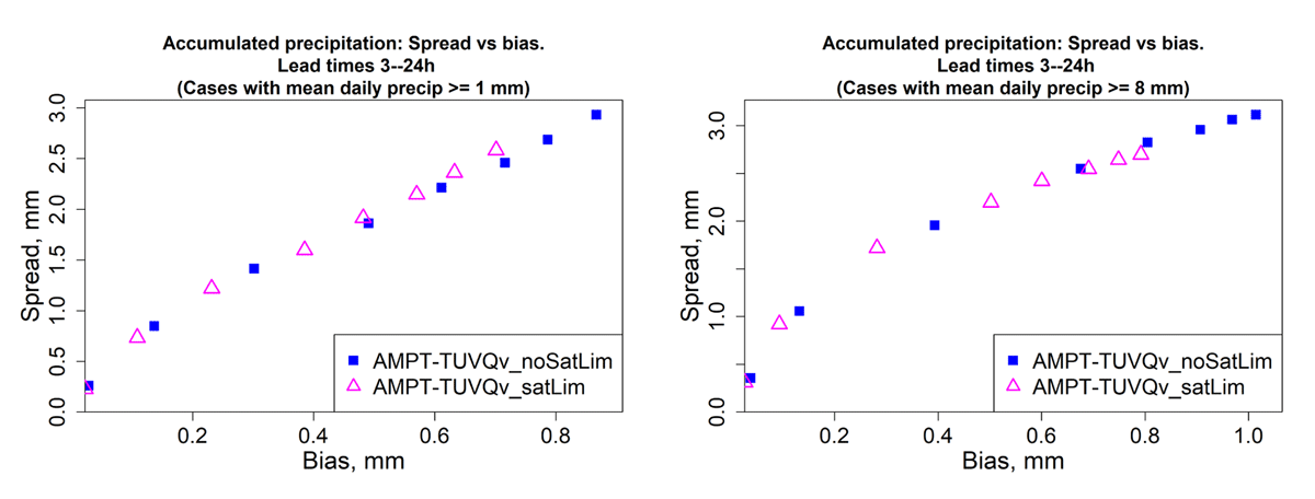
Figure 2
Impact of the supersaturation limiter on spread and bias of accumulated precipitation forecasts for lead times from 3 to 24 h. Averaging over cases with the mean (over the model domain) daily accumulated precipitation ⩾ 1 mm (left) and ⩾ 8 mm (right).
4.2 Roles of humidity and temperature perturbations
Here we compare three configurations of AMPT and the basic configuration of SPPT in terms of their impacts on the bias and the spread of the ensemble. In the AMPT-TUVQv configuration, T, u, v, qv fields were perturbed. In the AMPT-TUV configuration, only T, u, v fields were perturbed (that is, without humidity model perturbations). In the AMPT-UV configuration, only u,v fields were perturbed. With AMPT-UV, we found that the spread in the ensemble was somewhat too small. This led us to increase the amplitude multiplier κ in this configuration from its default value of 0.75 (see section 3) to 1.
Figure 3 shows bias-spread scatterplots for near-surface temperature. One can see that perturbing humidity on top of T, u, v did not change much neither the bias nor the spread (AMPT-TUV and AMPT-TUVQv performed similarly in these experiments). The other pair of schemes, SPPT and AMPT-UV, had significantly lower (in modulus) bias and spread. In dry conditions (the top left plot), SPPT had a smaller spread and bias-to-spread ratio than AMPT-UV. In wet conditions (the top right plot), SPPT and AMPT-UV performed similarly in terms of both spread and the bias-to-spread ratio, but the signs of the biases were different: negative for SPPT and positive for AMPT. In very wet conditions (the bottom plot), it was AMPT-UV that had the smallest bias-to-spread ratio while having nearly the same spread as SPPT.
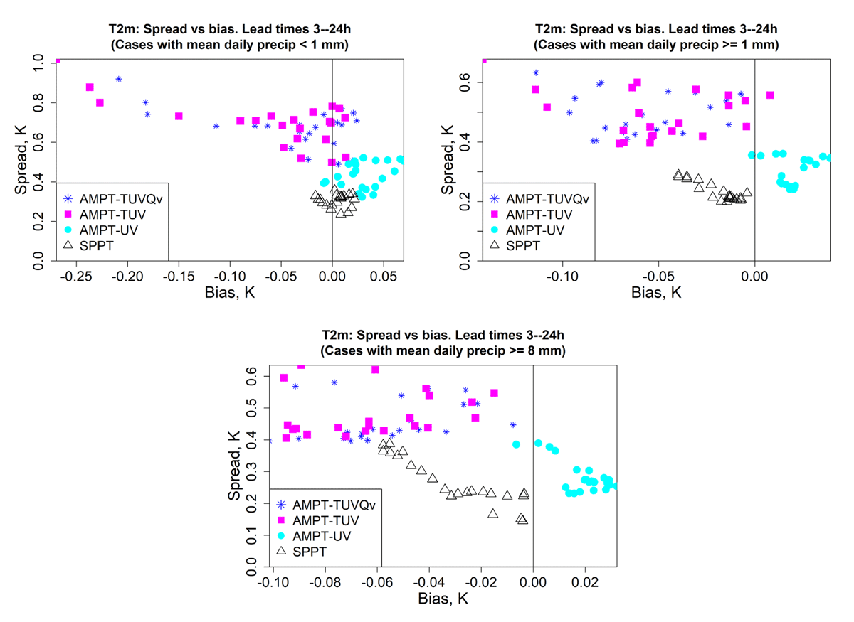
Figure 3
Spread vs bias of T2m forecasts for lead times from 3 to 24 h. Averaging over cases with the mean (over the model domain) daily accumulated precipitation <1 mm (top, left), ⩾ 1 mm (top, right), and ⩾ 8 mm (bottom).
Figure 4 shows bias-spread scatterplots for accumulated precipitation. In both wet (the left plot) and very wet (the right plot) conditions, the differences between the four schemes were more systematic than in Figure 3. Like in Figure 3, the magnitudes of precipitation bias and spread of SPPT and AMPT-UV were quite similar. Again, like for T2m, AMPT-TUV and AMPT-TUVQv had significantly greater (than SPPT and AMPT-UV) bias and spread, but unlike Figure 3, the bias-to-spread ratio for AMPT-TUV was significantly lower than for AMPT-TUVQv.
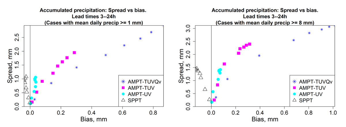
Figure 4
Spread vs bias of accumulated precipitation forecasts for lead times from 3 to 24 h. Averaging over cases with the mean (over the model domain) daily accumulated precipitation ⩾ 1 mm (left) and ⩾ 8 mm (right).
It is also worth noting that the precipitation biases in Figure 4 were negative for SPPT and positive for AMPT. Investigating mechanisms that lead a complex nonlinear model to generate biases of different signs under different zero-mean stochastic model perturbations would be interesting but is beyond the scope of this research.
We summarize findings from Figures 3 and 4 as follows.
The magnitudes of forecast bias and spread due to SPPT were similar to those due to AMPT-UV (i.e., AMPT without temperature and humidity perturbations).
The addition of temperature perturbations in AMPT (in AMPT-TUV) led to significantly greater spread but somewhat higher (i.e. worse) bias-to-spread ratio.
Perturbing humidity on top of T, u, v (in AMPT-TUVQv) led to a significant growth in spread for precipitation but at the expense of a significant degradation in the bias-to-spread ratio.
Thus, without temperature perturbations in AMPT (i.e. perturbing only u, v), we could not outperform SPPT in terms of spread. However, with humidity perturbations in AMPT (i.e., perturbing T, u, v, qv), forecast biases for precipitation were too large. Therefore, in the ensemble prediction experiments described in the next subsection, AMPT temperature (and winds) perturbations were switched on whereas humidity perturbations were switched off.
5 Testing AMPT in the ensemble prediction system
5.1 Setup
The general experimental setup described in section 3 applies to the experiments presented in this section with the caveat that there was no unperturbed member in the ensemble here. The results were verified against near-surface observations (about 40 stations) using the VERification System Unified Survey (VERSUS) developed within the COSMO consortium (Gofa et al., 2010).
The list of experiments and their basic features are presented in Table 1. In AMPT-SOIL, initial soil perturbations generated following section 2.4.4 were added to the respective fields of the initial-conditions ensemble members.
Table 1
List of ensemble prediction experiments.
| EXPERIMENT | MODEL PERTURBATIONS |
|---|---|
| NOPERT | None |
| SPPT | Atmospheric SPPT perturbations |
| AMPT-NOSOIL | Atmospheric AMPT perturbations |
| AMPT-SOIL | Atmospheric and soil AMPT perturbations |
Besides the four model perturbation schemes listed in Table 1, we also tested a hybrid of AMPT and SPPT. We expected that such a hybrid might lead to an improvement because SPPT and AMPT perturbations explore different volumes in phase space. Indeed, the direction of the SPPT perturbation vector (comprised of all model variables at a grid point or a grid column) exactly coincides with the direction of the physical tendency vector, Eq. (6). In contrast, the AMPT perturbation vector can have any direction because ξi are uncorrelated, see Eq. (10) and section 2.3.3, so it has nothing to do with the direction of the model’s physical tendency vector at all. Besides, the magnitude of the SPPT perturbation is proportional to the magnitude of the local physical tendency, which is never the case with AMPT. Somewhat surprisingly, we could not see any benefit from the hybridization of the two schemes (not shown), so we abandoned the hybrid. As suggested by an anonymous reviewer, this outcome might be caused by the smaller magnitude of SPPT perturbations, which therefore could not make a difference.
During the two-month trial, there were two cases (out of 59) in which one of the forecasts exhibited catastrophic instability. On March 15, three out of the four tested configurations ‘exploded’: NOPERT (in which, we recall, there were no model perturbations, only initial and lateral-boundary conditions were perturbed), SPPT, and AMPT-NOSOIL, whereas the most successful AMPT configuration, AMPT-SOIL, performed normally. On March 20, both AMPT configurations failed whereas NOPERT and SPPT were OK. These two cases were excluded from the forecast performance statistics. So, our experiments showed that numerical instability can happen with AMPT, but its frequency is nearly as low as with SPPT. A longer test period is needed to make a more precise statement.
In this section, we show verification scores for T2m forecasts averaged over the whole two-month period. Similar results were obtained for each of the two months separately (not shown). For near-surface wind speed V10m, verification results were, mostly, similar to those for T2m, except that soil perturbations had a significantly smaller impact on the wind speed than on temperature. This could be expected because perturbations of soil temperature and soil moisture directly impact surface fluxes of sensible and latent heat but not the flux of momentum. Due to the similarity of verification scores for V10m compared to T2m, we only display one typical plot for V10m below. We also present a comparison of AMPT and SPPT for upper-level fields.
With precipitation, the only statistically significant effect of AMPT was an increase in ensemble spread. This can be seen in the model-perturbations-only experiments reported above in section 4 (see Figure 4) and this was observed in the experiments described in this section (not shown). Other verification scores for precipitation forecasts were ambiguous because, on the one hand, the time period was rather dry and on the other hand, the observation network was too scarce to detect relatively rare and localized precipitation events (not shown).
In contrast to section 4, where the results were obtained by averaging over large samples (the whole spatial grid and two months of data), the ensemble forecasts examined in this section were verified against a relatively scarce observation network. This caused a larger statistical uncertainty and therefore required statistical significance testing, see Appendix B for methodological details. The default settings of the statistical significance calculations were as follows. We examined statistical significance of improvements due to AMPT-NOSOIL relative to SPPT because both schemes involved no soil perturbations and thus were comparable. We averaged the scores over all lead times up to 48 h to reduce statistical uncertainty. The significance level was set at α = 0.05. The number of bootstrap samples was 105. Along with the p-value of the above bootstrap test, pbootstrap, we also computed the p-value of the classical one-sided Student’s t-test, pStudent.
5.2 Accuracy of ensemble mean forecasts and reliability of probabilistic forecasts
Figure 5(left) shows root-mean-square errors (RMSE) of the T2m ensemble mean forecast (the upper bunch of curves). Each curve corresponds to a model perturbation scheme from the list in Table 1. One can see in Figure 5(left) that, excluding the initial transient (spinup) period of some 3 h (likely, due to imbalances in initial conditions), the RMSE had a prominent diurnal cycle with a broad minimum at night and a narrower maximum shortly after midday.
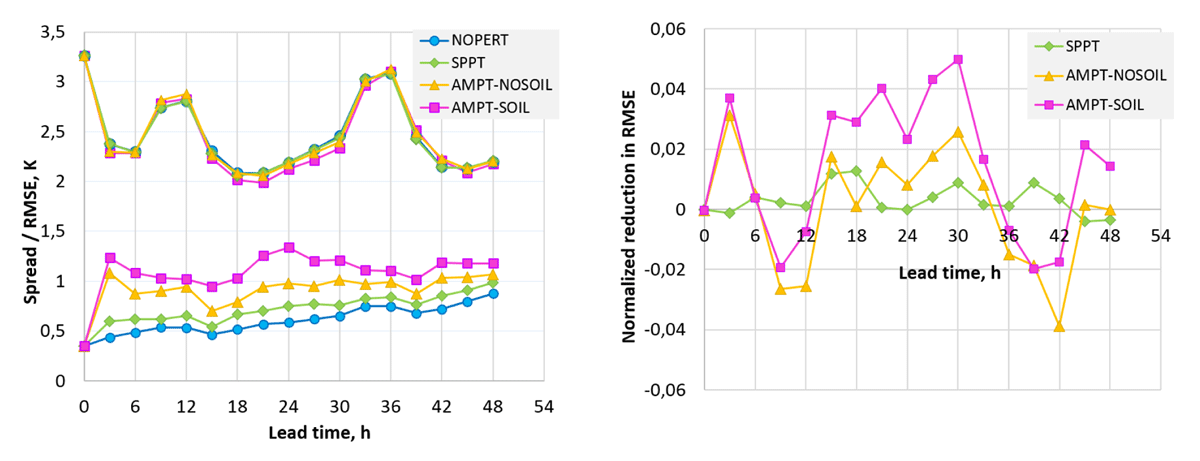
Figure 5
T2m. Left: RMSE of ensemble mean (the upper bunch of curves) and ensemble spread (the lower bunch of curves). Right: The normalized reduction in ensemble-mean RMSE, that is, (RMSENOPERT – RMSE)/RMSENOPERT, the higher the better.
To highlight the barely seen in Figure 5(left) differences between the curves in the upper bunch, Figure 5(right) displays the normalized reduction in the T2m ensemble-mean RMSE with respect to NOPERT, that is, (RMSENOPERT – RMSE)/RMSENOPERT. SPPT perturbations led to a slight overall reduction in RMSE. AMPT-NOSOIL perturbations gave rise to a more significant decrease in the T2m RMSE most of the time except for the rather short time period in the afternoon local time when the ensemble-mean forecast deteriorated. The effect of soil perturbations on the ensemble mean forecast looks positive: the RMSE reduction is seen to be nearly uniformly higher in the experiment AMPT-SOIL than in AMPT-NOSOIL. However, all these differences were not statistically significant at the 0.05 level. For near-surface wind speed, the results were similar, not shown.
The lower bunch of curves in Figure 5(left) shows the ensemble spread in T2m for the four schemes examined. One can see that the spread was somewhat too low with both SPPT and AMPT, though AMPT perturbations induced substantially greater spread than SPPT perturbations (this conclusion was valid for the spread in V10m as well, not shown). The advantage of AMPT-NOSOIL over SPPT in terms of spread was highly statistically significant: the p-values of both the bootstrap test and the Student’s t-test were less than 0.001. For all 8 weeks and all lead times, the forecast spread with AMPT-NOSOIL was substantially greater than the spread with SPPT. The advantage of AMPT-SOIL over SPPT is seen to be even bigger.
Note that in an ideal ensemble, its members are indistinguishable from the truth. Both members of such an ensemble and the truth can be viewed as independent draws from the same probability distribution. In particular, the expectation of any member equals the expectation of the truth. The standard deviation of any member at some point in space and time (let it be denoted by σ) is the same as the respective standard deviation of the truth. Then, the expected square of the ensemble spread (defined as the square root of the unbiased sample variance) equals σ2 by construction. At the same time, the expected square of the error in the ensemble mean (the mean-square error, MSE) equals , where N is the ensemble size (Fortin et al., 2014). Being averaged in space and time, the expected square of the ensemble spread becomes equal to . Correspondingly, the averaged in space and time MSE becomes . Thus, it is clear that for large ensembles, the root-mean-square spread should be very close to RMSE. For an ensemble of size N = 10 used in this study, RMSE should, on average, exceed the spread by , which is of course much smaller than the differences between the RMSE and the spread seen in Figure 5(left).
Another reason why forecast RMSE can be greater than ensemble spread is observation error. In complex terrain, the dominant source of error can be representativeness uncertainty, which accounts for the fact that observations can poorly represent grid-cell averaged fields provided by the model. We did not account for the contribution of observation error to RMSE.
It is worth mentioning that the variations in the RMSE as functions of lead time seen in Figure 5(left) are not accompanied by corresponding variations in the spread. The reason is that the diurnal-cycle variations in RMSE were largely caused by systematic forecast errors (biases). Indeed, verification results of COSMO model forecasts on different domains presented in (Rieger et al., 2021) show that the magnitude of diurnal variations in the forecast bias is between 1K and 2K, with a broad maximum at night and a narrow minimum in the afternoon. Stochastic zero-mean model perturbations, cannot, in general, represent model biases, implying that the forecast spread cannot reflect the contribution of the bias to the RMSE. Either the forecasts are to be debiased or a multi-physics/multi-model ensemble (in which different members have different biases) is to be used, see, e.g., Berner et al. (2015).
Higher in the atmosphere, the effects of AMPT were similar to what we found for the near-surface fields. Figure 6 shows the RMSE and spread for upper-level temperature and wind speed (averaged over four lead times: 12, 24, 36, and 48 h). RMSE was computed here with respect to the ECMWF analyses interpolated to the model grid. It is seen that AMPT produced a higher spread and nearly the same RMSE as SPPT. The superiority of AMPT over SPPT in terms of spread was statistically significant for both fields at all levels shown in Figure 6, with p < 0.001 for both the bootstrap test and Student’s t-test. It is interesting to note that for temperature, the RMSE and spread were maximal near the ground (where turbulence and small-scale disturbances due to orography are the strongest). For wind speed, on the contrary, both the RMSE and spread were the smallest at the lowest model levels. Their downward decrease was most pronounced in the surface layer (perhaps, because the wind speed itself is relatively low near the ground due to turbulent friction).
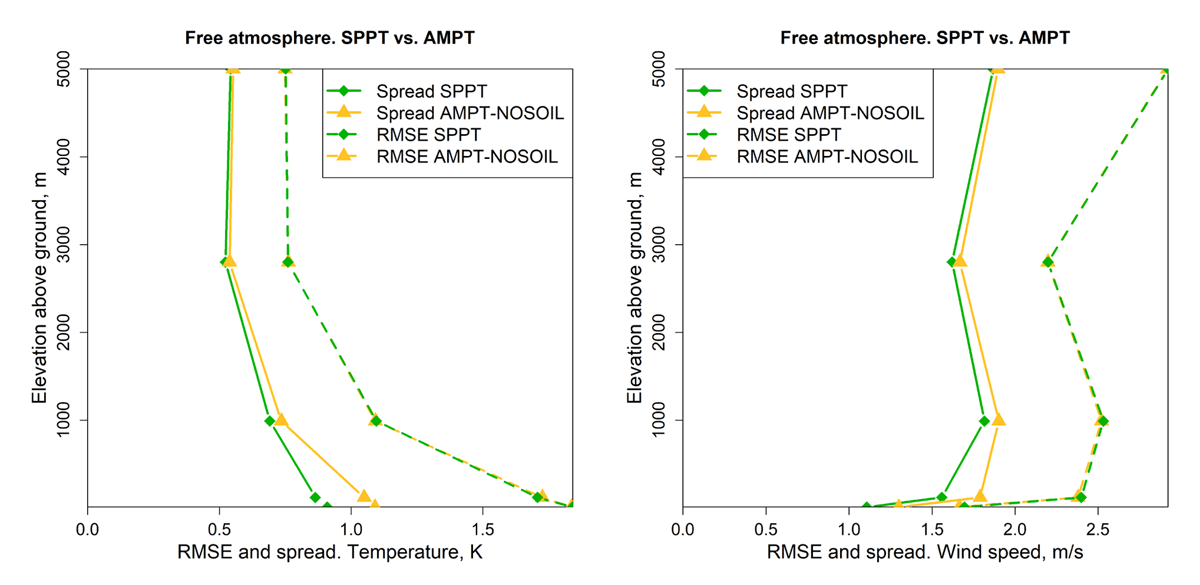
Figure 6
RMSE and spread for AMPT-NOSOIL vs. SPPT in free atmosphere.
Left: Temperature. Right: Wind speed.
If the spread is systematically and significantly different (say, lower, as in our experiments) than RMSE, then the conditional cumulative distribution function of the verification (truth, observation) xv given the ensemble cumulative distribution function Fe(x) of the model variable x, i.e., P(xv ⩽x | Fe) (where P stands for probability), is systematically different from Fe(x). This kind of inconsistency is known as lack of reliability of the probabilistic forecast (Toth et al., 2003). In these terms, Figures 5(left) and 6 demonstrate that AMPT perturbations are capable of significantly improving reliability of ensemble-based probabilistic forecasts compared to SPPT perturbations.
Figure 7 presents a more direct illustration of improvements in reliability brought about by AMPT-NOSOIL and AMPT-SOIL with respect to NOPERT and SPPT. It shows the reliability component of the Brier score2 for the (most populated) event T2m > 0°C. The improvement of AMPT-NOSOIL with respect to SPPT was statistically significant, pbootstrap = 0.05 (though pStudent = 0.07 did not reach the significance level of 0.05).
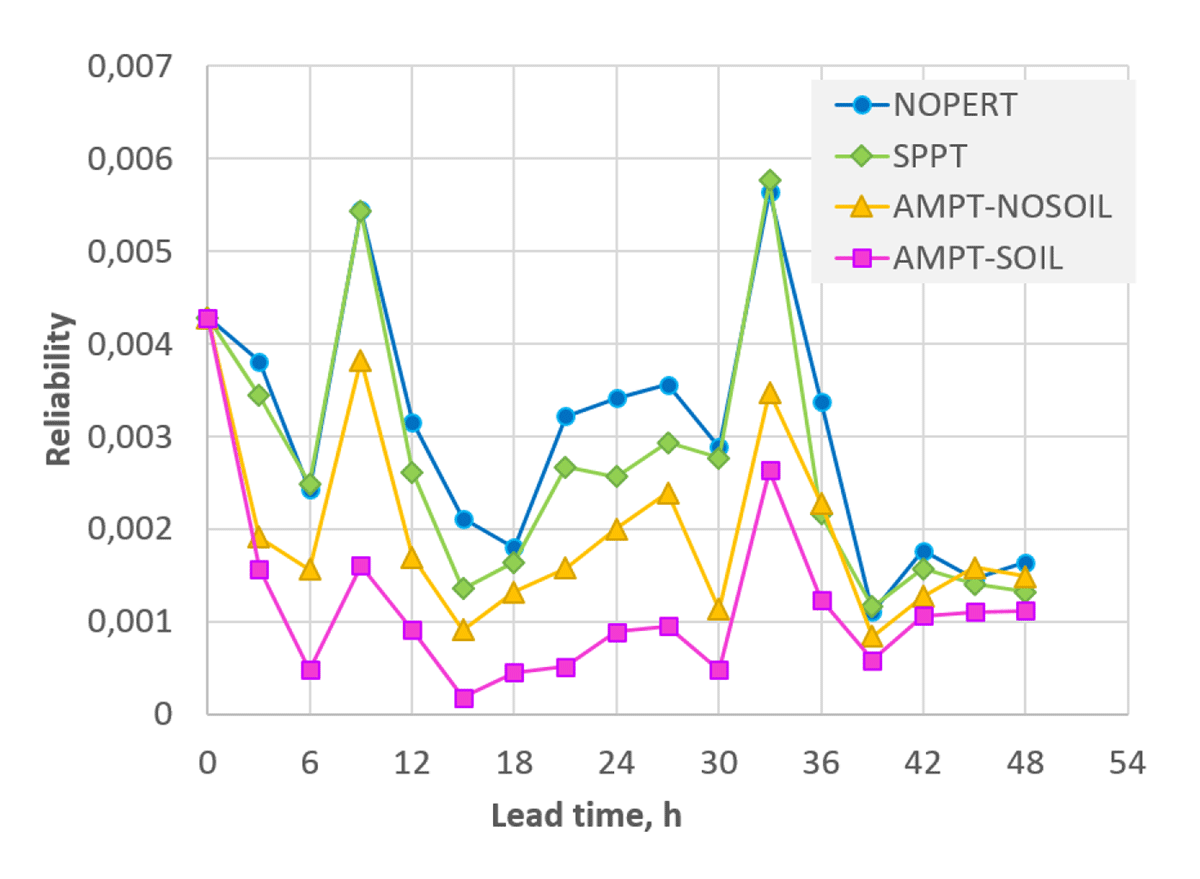
Figure 7
The reliability component of the Brier score for the event T2m > 0°C. The lower the better.
5.3 Resolution and discrimination of probabilistic forecasts
A reliable uncalibrated ensemble-based probabilistic forecast tells the user that if the ensemble variance (i.e., the spread squared) at some point in space and time equals some number d, then the expected MSE (RMSE squared) also approximately equals d. This is an important property expected from an ensemble. However, reliability alone does not fully characterize the quality of a probabilistic forecast. Indeed, the constant spread equal to the ‘climatological’ RMSE would imply a perfectly reliable forecast, which is, however, not much useful. The ensemble needs to generate sufficiently variable spread. If it does and if variations in the spread correspond to variations in the RMSE (the property known as resolution), then the ensemble can provide relevant information about the spatially and temporally variable RMSE.
One useful measure of resolution combined with reliability is the continuous ranked probability score (CRPS). Figure 8 displays CRPS for T2m. One can see that both SPPT and AMPT perturbations did improve CRPS (compared with NOPERT) while AMPT led to substantially greater improvements, especially with additional soil perturbations. The improvements of AMPT-NOSOIL compared with SPPT were statistically significant. The p-value of the bootstrap test computed following Appendix B was pbootstrap = 0.03. The p-value of the Student’s t-test was pStudent = 0.02. AMPT-SOIL performed a fortiori statistically significantly better than AMPT-NOSOIL.
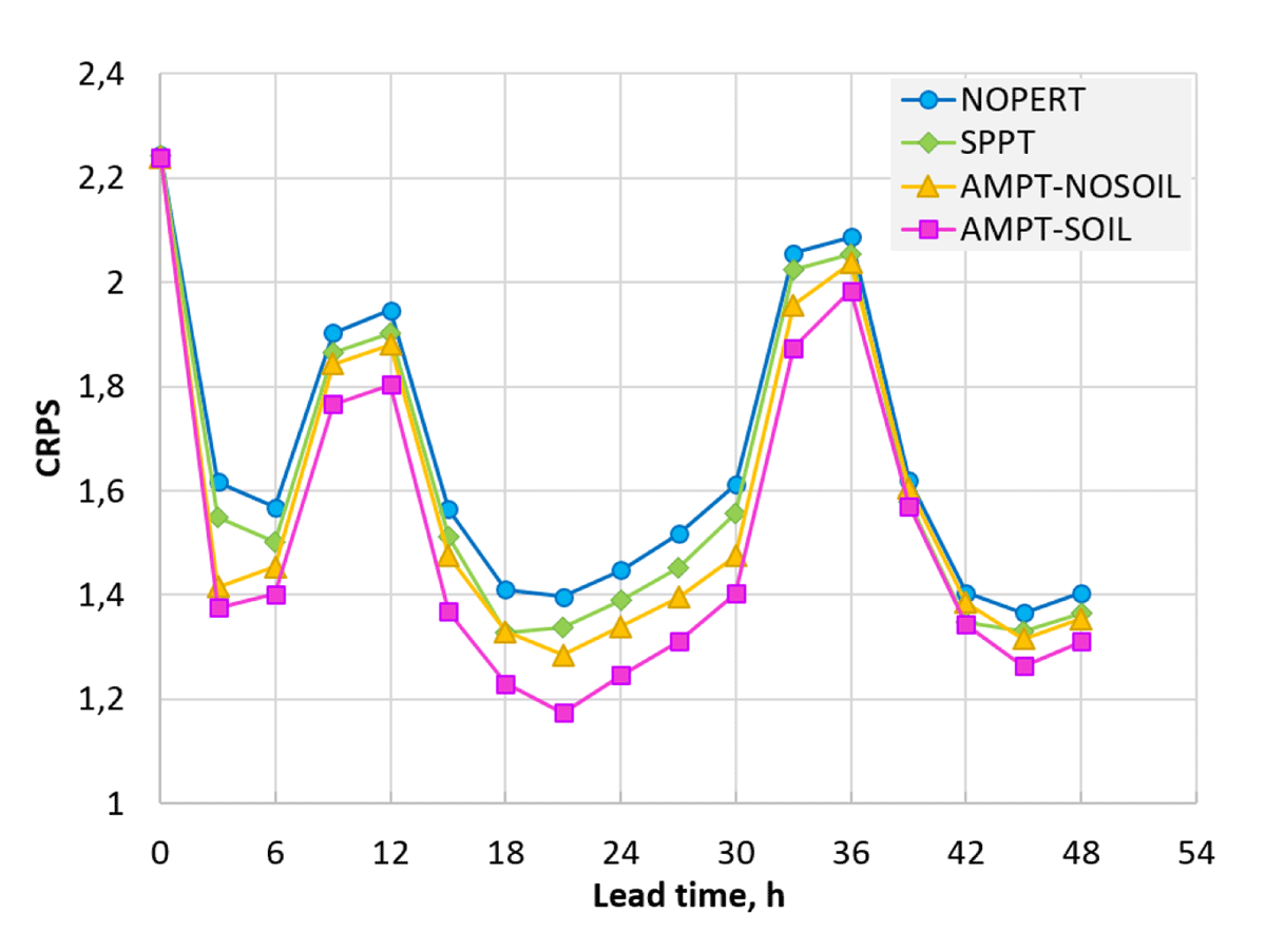
Figure 8
CRPS for T2m. The lower the better. Note that the y-axis does not start at 0.
Figure 9 displays CRPS for near-surface wind speed V10m. The impact of AMPT on the forecast performance in terms of V10m was weaker than on T2m but more stable, so the statistical significance of the advantage of AMPT-NOSOIL vs SPPT was stronger: pbootstrap < 0.001 and pStudent = 0.004. Soil perturbations contributed little to the forecast CRPS. We mentioned a reason for that in section 5.1. Why the impact of AMPT on wind was weaker (but more stable) than the impact on temperature in the settings without soil perturbations remains unclear.
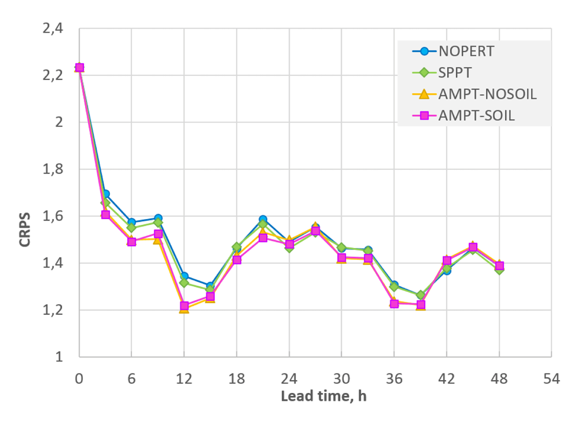
Figure 9
CRPS for V10m. The lower the better. Note that the y-axis does not start at 0.
Another popular measure of reliability and resolution is the Brier score, which, in contrast to CRPS, is computed for specific events. If the event is defined as x < θ (or x > θ), where x is the continuous model variable in question (say, temperature) and θ is a threshold, then CRPS is the integral of the Brier score over all possible θ (Hersbach, 2000). Therefore, Figure 8 implies that the Brier score integrated over all temperature thresholds is better with AMPT than with SPPT. To find out what happens for specific distinct thresholds, we selected several meteorologically relevant events () and verified the ensemble forecasts using the Brier score. AMPT did outperform SPPT for all these events, we show the results for the most populated event T2m > 0°C in Figure 10 (for near-surface wind speed, the results were similar, not shown). The improvements of AMPT-NOSOIL (and AMPT-SOIL as well) compared with SPPT were again statistically significant: pbootstrap = 0.03 and pStudent = 0.01. Similar results were obtained for near-surface wind speed, not shown.
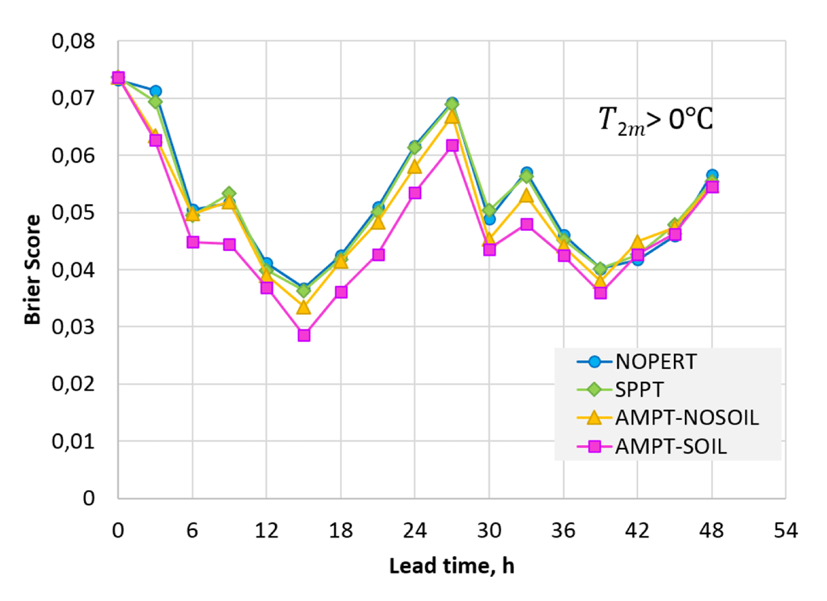
Figure 10
Brier score for the event T2m > 0°C. The lower the better.
We also examined the resolution component of the Brier Score. With the reliability component substantially improved, see Figure 7, the resolution component was barely changed or slightly reduced (i.e., degraded, not shown). As noted by Candille and Talagrand (2005), an increase in spread may lead to a degradation in resolution because a larger spread is more akin to the climatological spread, which yields no resolution. So, we state that AMPT substantially improved reliability without significantly degrading resolution.
As discussed above, the ability of a probabilistic forecast to predict the uncertainty in the forecast can be measured by reliability and resolution through the conditional distribution of the verification xv given the ensemble cumulative distribution function Fe(x), i.e., p(xv | Fe) (where p stands for probability density). The reciprocal and complementary view on the accuracy of a probabilistic forecast is through p(Fe | xv), i.e., conditional on verification. The capability of a probabilistic forecast to concentrate the probability mass close to the observed xv (thus, discriminating between different outcomes xv) is called discrimination (e.g., Wilks, 2011).
Discrimination is commonly assessed using the Relative Operating Characteristic (ROC) defined for a specific meteorological event and, more succinctly, using the area under the ROC curve (ROC area). Figure 11 shows the ROC area for the event T2m > 0°C (similar results were obtained for the two other events, T2m < –5°C and T2m > 5°C, not shown). From this figure, we see that AMPT did outperform SPPT. Our statistical significance tests showed that the advantage of AMPT-NOSOIL over SPPT in terms of ROC area was statistically significant: pbootstrap = pStudent = 0.01. As AMPT-SOIL is seen in Figure 11 to be almost uniformly better than AMPT-NOSOIL, we conclude that AMPT-SOIL was statistically significantly more skilful for near-surface temperature than SPPT, too. For near-surface wind speed, the results were mixed (not shown).
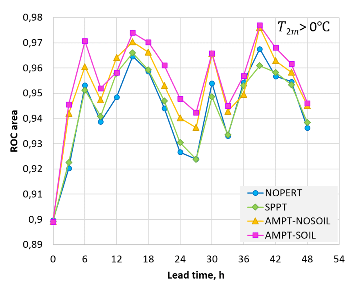
Figure 11
ROC area for the event T2m > 0°C. The higher the better. Note that the y-axis does not start at 0.
A few remarks regarding Figure 11 are in order. First, the overall level of the ROC area score was quite high (its perfect value is 1 whereas a value less than 0.5 indicates no skill) so the probabilistic forecasts in question were quite skillful. Second, as with many other plots above, the ensemble forecasts were the worst at zero lead time. This was, most likely, caused by the poor quality of the initial ensemble. Finally, we note that the ROC area is known to be insensitive to the degree of reliability and cannot be improved by calibration of a probabilistic forecast (e.g., Wilks, 2011). Therefore, the superiority of AMPT-SOIL over SPPT and NOPERT in terms of ROC area implies that AMPT did not just inflate spread (which could be done by calibration), it can yield ‘good spread’ in the sense of Eckel and Mass (2005), meaning greater spread when and where it is relevant.
5.4 Summary of ensemble prediction results
For near-surface temperature forecasts, atmospheric AMPT perturbations gave rise to statistically significant improvements (compared to SPPT) in the performance of the ensemble prediction system — in terms of spread-skill relationship, CRPS, Brier score, and ROC area. In terms of RMSE of the ensemble-mean forecast of near-surface temperature, the effects of AMPT were mixed. For near-surface wind speed forecasts, the effects of the atmospheric AMPT were similar to but weaker than the effects on near-surface temperature forecasts. Soil AMPT perturbations imposed in addition to atmospheric AMPT perturbations led to nearly uniform further improvements in the ensemble performance for near-surface temperature and smaller improvements in near-surface wind speed. The impact of AMPT on precipitation forecast scores was mixed.
In the free atmosphere, AMPT consistently generated bigger spread than SPPT, without degrading RMSE. The positive effect of AMPT, though, decreased away from the surface. We recall that our focus in this study was on the near-surface fields, so we did nothing to increase the spread induced by AMPT in the free atmosphere.
6 Conclusions
A new technique called Additive Model-uncertainty perturbations scaled by Physical Tendency (AMPT) has been proposed. AMPT addresses some issues of the wide-spread SPPT scheme. First, in contrast to SPPT, AMPT can generate perturbations with significant magnitude even at grid points where the model physical tendency happens to be spuriously small or is small due to cancellation of contributions from different physical parametrizations. Second, AMPT improves on the SPPT’s unphysical perfect correlations of perturbations between different model variables and in the vertical. Third, due to the non-local link from the model fields to the scaling physical tendency, which determines the magnitude of AMPT perturbations, the SPPT’s ban on sign reversal of the physical tendency, Eq. (5), is removed in AMPT. This enables AMPT to generate significantly greater perturbations than SPPT without causing instabilities.
Taking the unperturbed model run to introduce state-dependence in model perturbations for ensemble members is discussed. This approach breaks the positive feedback loop from the model state to perturbations and then back to the model state at a later lead time, therefore, it can be used to maintain stability of ensemble forecasts perturbed in a state-dependent manner. We found in this research that just relaxing the pointwise dependence of the model perturbation magnitude on the model state (by using a spatial moving average of the magnitude of physical tendency and by updating it less frequently than each model time step) helped much in preventing instabilities.
AMPT employs the Stochastic Pattern Generator (SPG, Tsyrulnikov and Gayfulin, 2017) to generate four-dimensional random fields with tunable spatio-temporal correlations (but can be used with any pattern generator). The random fields generated by SPG to perturb different model fields are mutually independent. They are scaled by the area-averaged modulus of physical tendency and added to the model fields at every model time step. AMPT perturbations of three-dimensional atmospheric model fields of temperature, pressure (computed from temperature perturbations via hydrostatics), wind, humidity, and three-dimensional soil fields (temperature and moisture) were imposed and their effects on convection-permitting ensemble forecasts (based on the COSMO forecast model) were examined.
Practically, AMPT performed better than SPPT in our ensemble prediction experiments but at the expense of being computationally more expensive than SPPT. The bigger cost of AMPT was mostly because the AMPT’s random patterns are three-dimensional (in the atmosphere), as opposed to two-dimensional random patterns in SPPT. In two dimensions (in the horizontal, soil perturbations), the cost of running AMPT was negligibly small. The overhead of running AMPT with the perturbed three-dimensional T,u,v fields (as well as p, TSO, and WSO) was about 10% of the time of running the COSMO model itself. There were three main computer-intensive parts of AMPT. First, the spectral SPG solver, which was optimized and parallelized, was responsible for about 25% of the total burden of AMPT. Second, the three-dimensional fast Fourier transform (FFT) took another 25% of computer time. FFT was only partly optimized and done with an old legacy code. The third computer intensive part was the computation of the scaling physical tendencies and spatial interpolations. This part was not parallelized at the time of writing this paper. As a result, AMPT was about 10 times more expensive than SPPT, but the gap can be reduced by a factor of three after the AMPT code is fully optimized in preparation for an operational application.
Another difference between AMPT and SPPT is that AMPT has many more parameters. On the one hand, this can be viewed as a disadvantage because AMPT requires more effort to tune them. On the other hand, all the AMPT parameters have clear physical meaning and are set to meaningful default values. This offers the AMPT user a choice: either to set the parameters to their default values indicated in section 3 or to tune some of the parameters taking into account specifics of a particular application.
It is also worth noting that AMPT suffers from a lack of physical consistency even to a greater extent than SPPT since AMPT perturbations are not balanced. We argue that this might not be a problem because of a small magnitude of model perturbations introduced every model time step so that the model manages to balance them itself. Experimentally, we found no indications of problems related to the lack of balance in AMPT perturbations.
The main findings of the study are the following.
Humidity perturbations generated significant ensemble spread in precipitation forecasts but led to a high bias-to-spread ratio. For this reason, AMPT was systematically tested without humidity perturbations.
Withholding temperature perturbations led to a substantial reduction in the bias and in the bias-to-spread ratio, but at the expense of a substantial reduction in spread as well. For this reason, temperature (and pressure) were included in the list of perturbed model fields in the final ensemble prediction experiments.
In ensemble prediction experiments, it was found that AMPT was much more effective in generating spread in the ensemble than SPPT, thus considerably improving reliability of the ensemble. This was the case for the upper-air fields as well as for the near-surface fields.
Most probabilistic ensemble verification scores for near-surface temperature and wind speed were improved due to atmospheric AMPT perturbations as compared with SPPT (at the statistical significance level of 0.05).
Impacts of AMPT on the root-mean-square errors of the ensemble-mean temperature and wind speed forecasts were mixed (compared with SPPT). This held for free-atmosphere as well as near-surface variables.
AMPT perturbations of soil moisture and soil temperature significantly improved deterministic and probabilistic verification scores for near-surface temperature and had little effect on near-surface wind speed.
Probabilistic verification of ensemble forecasts in terms of precipitation gave mixed results, perhaps, due to an insufficient number of precipitating events during the time period examined and scarcity of the observation network.
The technique can be further developed in the following directions. First, it looks reasonable to introduce state-dependence not only in the magnitude of perturbation fields but also in their spatial and temporal scales. This will require a non-stationary (in space and time) stochastic random field generator (e.g., based on the technique proposed in Tsyrulnikov and Rakitko (2019)) and a method to specify the non-stationarity patterns. Second, in its current formulation, AMPT takes the net physical tendency as input but it can be used at the process level as well, i.e., for the output of each parametrization scheme separately. Third, switching from perturbations of tendencies to perturbations of fluxes looks as a promising way to achieve physical consistency. Finally, we note that AMPT can be used in data assimilation as well as in ensemble prediction systems: in the atmosphere, in the soil, and also in the ocean.
Appendices
A Additive and multiplicative perturbations
This Appendix contains remarks on the suitability of the term ‘additive’ in the acronym AMPT.
In stochastic systems theory, the term ‘additive noise’ denotes a perturbation that does not depend on the system state. If the perturbation is a function of the system state, it is called multiplicative, e.g., Fuchs (2014, sec. 6.5). We recall that in ensemble prediction, an ensemble member can be viewed as a numerical solution to the stochastic dynamic equation of the unknown, random truth (system state), e.g., Tsyrulnikov and Gayfulin (2017, Eq.(1.3)): dx/dt = F(x) – ξ (where x is the truth, F is the forecast-model operator, and ξ is the random model perturbation). So, the model perturbation is multiplicative if it is a function of x (the state of the ensemble member on which the model perturbation is imposed) and additive if it does not depend on x.
With SPPT, the model perturbation at some point in space and time, (s, t), is proportional to the physical tendency P(x(s, t)), where x is the state of the ensemble member, Eq. (6). Therefore, the SPPT perturbation in each model variable i is a function of x and thus is multiplicative:
With AMPT, if the scaling tendency is taken from the control (unperturbed) run, so that , the perturbation ceases to depend on x:
it only depends on the known initial conditions of the control run. Thus, the AMPT perturbation is indeed additive in the setting in which the scaling physical tendency is taken from the control model run.
B Methodology of testing statistical significance
Here we describe how we calculated statistical significance of improvements due to AMPT in ensemble prediction experiments presented in section 5.
Let us test the hypothesis that a verification score ψ is greater for scheme 1 than for scheme 2. More precisely, we are going to compare the scores ψ1 and ψ2 that could be obtained from a very large sample of forecasts, whilst having their unbiased estimates and obtained from smaller samples. That is, the hypothesis to be tested is . The default ‘null’ hypothesis states that there is no difference between the two schemes: H0: ψ1 = ψ2.
Since atmospheric states are correlated in time and forecast errors depend on the atmospheric flow, forecast errors are also temporally correlated (dependent). Accounting for these time correlations would complicate statistical hypothesis testing, so for simplicity, we employ the following approach. We divide the whole two-month period into n=8 weeks and compute the score ψ for each of the two schemes for each week separately, getting the respective sequences and (for j = 1, 2, …, n) and their differences . We treat as (observed) realizations of the respective random variables δj. Assuming that temporal dependencies in δj decay on a time scale shorter than one week, we regard δj as a sample of statistically independent and identically distributed random numbers.
Informally, if are mostly positive, we tend to believe that , meaning that the hypothesis H we are testing is true. Formally, we reject H0 (and thus accept H) if , where the overbar denotes sample averaging, is sufficiently small. This means that if, under H0, the probability of the observed (and more extreme) deviation of away from zero is small, then the data we have are, likely, not consistent with H0. Specifically, we select a significance level, α, and reject H0 if the above probability p (known as the p-value) is less than α.
To compute p we need to know the probability distribution of δj under H0. This can be easily done using an approach to statistical inference known as bootstrap. In its simplest flavor, bootstrap postulates that the data distribution (i.e., the distribution of δj) equals the empirical distribution (which is concentrated at the observed data, in our case, ). However, this setup cannot be directly applied here because H0 assumes that whereas the empirical distribution is, likely, biased (). Following Efron and Tibshirani (1994, ch.16), to define the bootstrap distribution, we shift the empirical distribution so that it has zero mean. Then, we proceed as usual, sampling (with replacement) from this discrete distribution (concentrated with equal probabilities at the points ), compute the mean in each bootstrap sample, , and calculate the fraction of bootstrap samples in which . This fraction is the estimate of the p-value.
Data availability statement
The dataset on which this paper is based is too large to be retained or publicly archived with available resources. Documentation and methods used to support this study are available from the first author. The Fortran source code of SPG is available from https://github.com/gayfulin/SPG. Reproducible R code that realizes the methodology of statistical significance testing (presented in Appendix B), along with raw data, can be found at https://github.com/cyrulnic/AMPT.
Notes
[1] In the experiments described below, the mean absolute magnitudes of AMPT perturbations per time step were as follows (at 8 a.m. local time). Temperature: somewhat less than 0.001 K in the lower 3-km tropospheric layer and much less above it. A horizontal wind component: from 0.015 m/s near the ground to 0.0001 m/s at 3 km height and even less above 3 km.
[2] The reliability component of the Brier score is a weighted mean-square difference between the predicted event probabilities (where k labels the discrete values of the forecast probability obtainable from a finite-size ensemble) and the respective observed frequencies of the event for all cases when the probability was forecast.
Acknowledgements
We are grateful to T.Paccagnella and A.Montani, who provided us with initial and boundary conditions for our forecast ensemble. We would like to thank members of the COSMO Working Group on Predictability and Ensemble Methods for many fruitful discussions. V.Volkova assisted with the ensemble forecast verification in the free atmosphere. A.Kirsanov and A.Bundel kindly helped us to use the VERSUS verification tool. We also thank D.Blinov for assistance in working with the COSMO model. Valuable comments of two anonymous reviewers led to significant improvements of the manuscript. The study has been conducted under Tasks 1.1.1 and 1.1.4 of the Scientific Research and Technology Plan of the Russian Federal Service for Hydrometeorology and Environmental Monitoring.
Competing Interests
The authors have no competing interests to declare.
Author contributions
All authors contributed to the study conception and design. Michael Tsyrulnikov wrote the manuscript. Elena Astakhova performed ensemble prediction experiments and verification. Dmitry Gayfulin wrote the program code and conducted preliminary sensitivity tests. All authors commented on previous versions of the manuscript. All authors read and approved the final manuscript.